Audio Signal Classification Using Deep Learning

Abstract

Audio signal classification plays a significant role in various real-world applications such as speech recognition, environmental sound analysis, and music genre identification. Traditional approaches often depend on manually extracted features, which may not capture the full complexity of audio data. This paper presents a deep learning-based method for automatic classification of audio signals using a One-Dimensional Convolutional Neural Network (1D-CNN) and a Recurrent Neural Network (RNN). The CNN model is utilized to extract spatial features from spectrogram representations, while the RNN model effectively captures temporal dependencies within the audio sequences. Both models were trained and evaluated on a labelled dataset, and their performance was compared using metrics such as accuracy, precision, probability of detection (POD), and F1-score. The experimental results demonstrate that CNN has achieved high classification accuracy compared to RNN, with CNN excelling at spatial feature extraction and RNN providing temporal feature learning. The proposed approach confirms that deep learning models can significantly enhance the performance and reliability of audio signal classification systems.

Introduction

Audio signal classification plays a crucial role in numerous applications, including speech recognition, environmental sound detection, music genre identification, and digital forensics. Audio signals contain both temporal and spectral information, making their accurate classification a challenging task. Conventional machine learning techniques, such as Support Vector Machines (SVMs) and Hidden Markov Models (HMMs), rely on handcrafted features including Mel-Frequency Cepstral Coefficients (MFCCs) and spectral centroids. These features provide limited representational capacity and are insufficient to effectively model the complex, non-linear, and time-varying characteristics of real-world audio signals [1]. Deep learning has recently gained prominence in audio signal processing by enabling end-to-end learning from raw or time–frequency representations. In particular, Convolutional and Recurrent Neural Networks effectively capture spectral characteristics and temporal dependencies in audio signals. CNNs effectively capture local spatial patterns in spectrograms, whereas RNNs, particularly long short-term memory (LSTM) and gated recurrent unit (GRU) variants, model long-term temporal dependencies in audio signals [2]. Rakesh Kumar, et al. [3] developed an intelligent audio signal processing system for rainforest species identification using CNN and LSTM networks, achieving accuracies of 95.62% and 93.12%, respectively. A hybrid CNN–LSTM model achieved 97.12% accuracy with reduced log loss, demonstrating the complementary nature of convolutional and recurrent architectures. Similarly, Meenu Gupta, et al. [4] implemented CNN and RNN models for environmental sound classification, reporting superior accuracy compared to traditional classifiers. In the field of music information retrieval (MIR), Pons, et al. [5] reviewed the application of deep learning models for music signal processing and highlighted CNNs’ ability to learn timbral and rhythmic representations directly from spectrograms. Kim, et al. [6] utilized bidirectional RNNs to enhance rhythm and melody recognition, demonstrating improved temporal modeling performance. Bhangale and Kothandaraman, et al. [7] emphasized that combining CNN and RNN models results in robust systems capable of handling various audio domains efficiently. Furthermore, deep learning techniques have found application in digital audio forensics, where they aid in identifying recording environments and microphone types. Qamhan, et al. [8] presented a CNN-based forensic audio classifier that discriminates recording conditions and acoustic environments using spectro-temporal features, demonstrating the effectiveness of deep learning architectures in forensic and audio authentication tasks. This work evaluates CNN and RNN-based models for audio signal classification to improve accuracy under background noise and varying recording conditions. The CNN extracts spectral features from spectrograms, while the RNN models temporal dependencies in sequential audio data. Both models are evaluated on a labeled dataset using accuracy, precision, probability of detection (POD), and F1-score [18-24]. The results indicate that the CNN has excelled in spatial feature learning and the RNN excels in temporal feature learning.

An abuser is defined as an individual who is habitual or dependent to drug resulting in harm to physical and psychological heath with social relationships or negative impacts to the community. In many developing nations, particularly across the Africa and Asia, tramadol was originally perceived as a safer option against other drugs due to low side effects. It has been observed that over the past decades, there has been a steady increased in misuse, dependence and illegal trafficking of tramadol (Figure 1).

Methodology

The architecture of CNN and RNN models for audio signal classification has been discussed here. The proposed model is designed to learn discriminative audio feature patterns directly from a structured dataset and map them to their corresponding genre classes through supervised training, thereby improving classification accuracy and robustness.

Architecture of one-dimensional CNN (1D-CNN)

The 1D-CNN model is designed to extract spatial feature representations from sequential numerical data. It processes one-dimensional sequences, making it suitable for time-series data such as music signal attributes. The convolutional layers learn local patterns within the input vector, such as rhythm, tempo, and harmonic structure correlations. The convolution operation can be mathematically expressed as:

Where $Y_m^{(k)}$ represents the output feature map, X_m represents the 1D input audio, $H_i^{(k)}$ represents the kernel values [18-24], k represents the number of kernels, j represents the kernel size, f represents the Rectified linear unit (ReLU) activation function, and Bm represents the bias [18-24]. The output of the convolutional layer was passed through the pooling layer to reduce the dimensionality of the feature map. Here, the max-pooling technique was employed [18-24]. The output of the pooling layer is given by:

Where X_m represents the 1D input and Y_m represents the pooling output. The output of the final pooling layer was flattened and given to the fully connected layer [18-24]. The output of the fully connected layer is given by:

Where Y_m denotes the output of the fully connected layer, f denotes the ReLU activation function, W_u denotes the weight values [18-24], X_q denotes the 1D data obtained through the flatten layer, B_m/sub> represents the bias, and n denotes the number of neurons [22-24]. The resulting feature representation is then passed to the output layer for multiclass classification. The output layer consists of five neurons corresponding to the target classes, and a softmax activation function is applied to produce the final class probability distribution [18-24]. The expression for the softmax function is given by:

Where Y_k represents the output, Xk represents the input, and n represents the number of neurons [18-24].

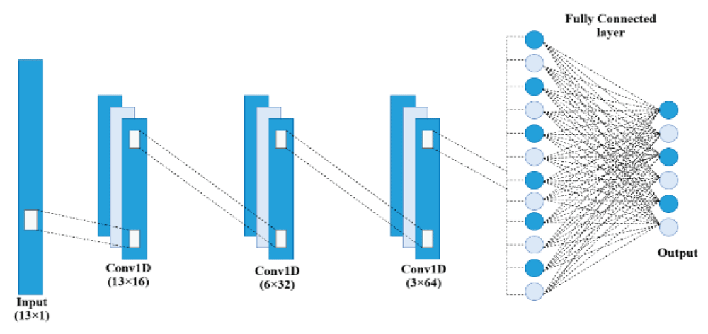
In Figure 1, the 1D CNN model consists of 16, 32, 64 kernels [18-24] in the 1st-3rd convolutional layers. The size of the kernel in each convolutional layer is one. The 1D-CNN model takes the input as 13 features and performs the audio signal classification task [18-24]. Pooling layers were employed subsequently after each convolutional layer in the 1D-CNN model. The output of the final pooling layer is flattened and further passed through the fully connected layer and then to the output layer to produce the final result [18-24].

Figure 1: Structure of tramadol, C₁6H25NO2.

Architecture of simple RNN

The Simple RNN model is designed to capture temporal dependencies and sequential relationships in the dataset. It maintains an internal memory of previous feature states, allowing it to learn time-related transitions in audio features such as rhythm progression and beat consistency. This makes RNN suitable for tasks involving sequence learning and contextual understanding [2]. At each time step t, the RNN computes its hidden state ht and output y_t using the following equations:

$y_t=Softmax(W_y{h}_t+c)$ (6)

In both Eqns 5 and 6, Wh, Wx, and Wy are weight matrices, and b and c are biases [2]. Wh represents the weight between the hidden-hidden state, and W_x represents the weight between the input-hidden state [2]. Similarly, Wy represents the weight between the hidden-output state. b represents the bias between the input-hidden state, and c represents the bias between the hidden-output state [2]. f represents the non-linear activation function, typically the hyperbolic tangent activation function [2]. The expression for the tanh hyperbolic activation function is given by

$f(x)=\text{tanh}(x)=\frac{e^x-e^{-x}}{e^x+e^{-x}}$ (7)

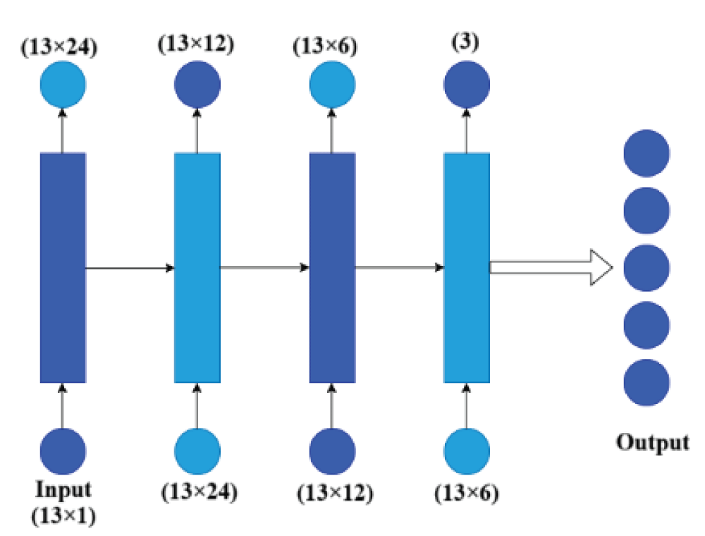
In Figure 2, the simple RNN model consists of 24, 12, 6, and 3 neurons in the 1st-4th RNN layers [2]. The simple RNN model takes the input as 13 features and performs the audio signal classification task. The output of the final RNN layer is flattened and further passed through the output layer to produce the final result. In the output layer, the softmax activation function was employed to get the output [18-24].

Figure 2: Proposed Simple RNN Architecture for Audio Classification.

Dataset preparation, results, and discussions

The dataset used in this study consists of musical audio features stored in CSV format taken from the Kaggle repository (https://www.kaggle.com/datasets/undefinenull/million-song-dataset-spotify-lastfm). Each record represents a music sample with attributes such as tempo, danceability, energy, loudness, and valence, among others. The time signature variable is chosen as the target variable. The data were normalized to ensure a uniform scale across features and were divided into training and testing subsets, with 75% of the data for training and 25% for testing. Both the 1D-CNN and RNN models use the categorical cross-entropy loss function, suitable for multi-class classification. The performance metrics considered for the audio signal classification task were accuracy, precision, POD, and F1-score. The model performance was evaluated using the following formulations.

1. Accuracy (A): the metric accuracy is defined as the ratio of the sum of true positive and true negative samples to the sum of all samples [18-24]. (TP-True Positive, TN-True Negative, FP-False Positive, FN-False Negative).

$A=\frac{TP+TN}{TP+TN+FP+FN}$ (8)

2. Precision: the metric precision is defined as the ratio of label TP to the sum of labels TP and FP [18-24].

$PPV=\frac{TP}{TP+FP}$ (9)

3. Probability of detection (POD): the metric POD is defined as the ratio of label TP to the sum of labels TP and FN [18-24].

$POD=\frac{TP}{TP+FN}$ (10)

4. F1-Score: the metric F1-score is defined as the ratio of twice the label TP to the sum of twice the label TP, and labels FP and FN [18-24].

$F1-score=\frac{2*TP}{2*TP+FP+FN}$ (11)

Collectively, these metrics offer a comprehensive evaluation of the effectiveness of each model in audio signal classification. The performance metrics obtained from 1D-CNN and Simple RNN models on the test set are as follows. The performance metrics are shown for Class-4 because the majority of the predictions belong to Class-4 in the case of the 1D-CNN model, whereas the simple RNN model has performance metrics for Class-3. After all, the majority of the predictions come under Class-3.

From Table 1, it can be said that the 1DCNN model has a precision of 0.75, a POD of 0.86, and an F1-score of 0.80 [18-24]. The overall accuracy of the 1DCNN model is 0.86 [18-24]. The results are summarized in Tables 1 and 2 for both 1D-CNN and Simple RNN models.

From Table 2, it can be said that the RNN model has a Precision of 0.87, a POD of 0.09, and an F1-score of 0.01 [18-24]. The overall accuracy of the RNN model is 0.09 [18-24]. From both Table 1 and Table 2, it can be said that the 1D-CNN model has higher accuracy compared to the simple RNN model. This indicates that CNN is performing the audio signal classification task much better compared to the simple RNN model. The F1-Score obtained from the 1D-CNN model is also much higher compared to the simple RNN model. However, the simple RNN model has higher precision and lower POD, whereas the 1D-CNN model has lower precision and higher POD. The accuracy and loss results obtained from the 1DCNN model on the training and validation sets are as follows.

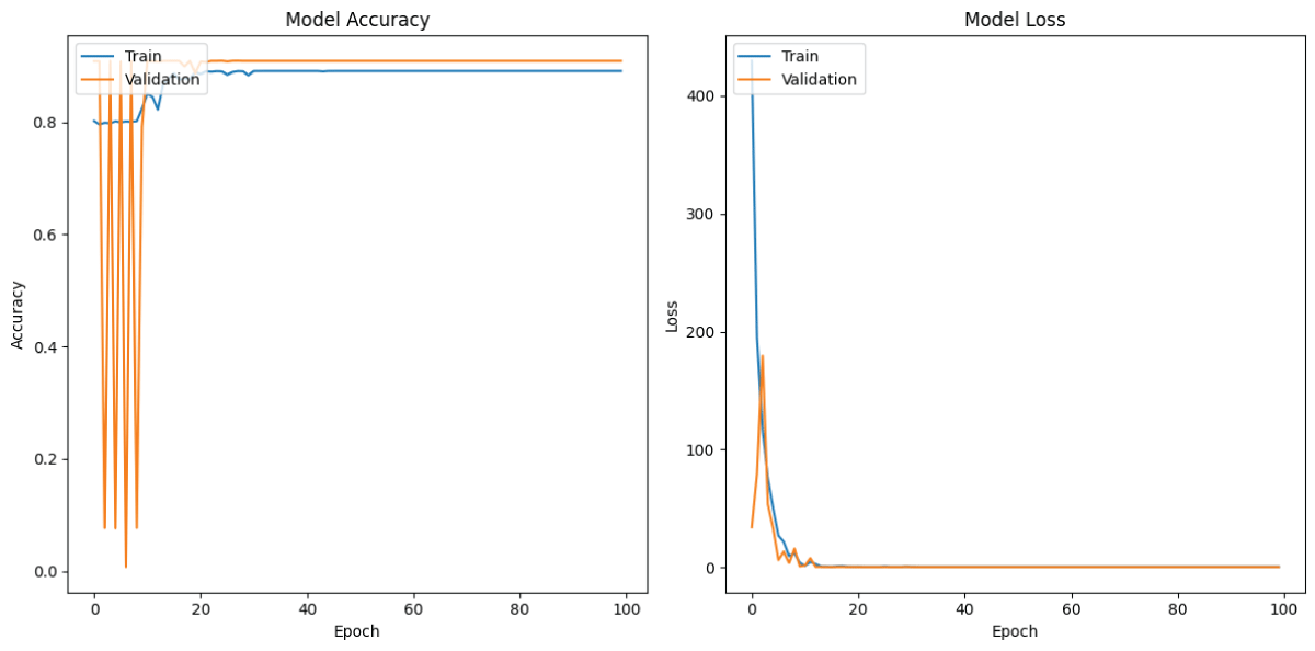
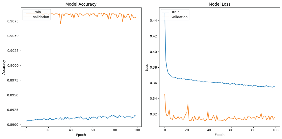
Figure 3 (a) shows the training and validation accuracy of the 1D-CNN model over 100 epochs [18-24]. The training accuracy gradually improves and stabilizes around 89%, while the validation accuracy reaches about 91%. The close values between them indicate good generalization and effective learning by the model without overfitting [18-24]. Figure 3 (b) shows the training and validation loss of the 1D-CNN model over 100 epochs [18-24]. The loss decreases sharply during the initial epochs and stabilizes near zero after 15 epochs. Both training and validation losses follow a similar trend, indicating efficient learning and minimal overfitting in the model [18-24].

Figure 3: Loss and Accuracy graphs of 1D-CNN model (a) Training and Validation Accuracy from 1D CNN model (b) Training and Validation Loss from 1D CNN model

The accuracy and loss results obtained from the Simple RNN model are as follows.

Figure 4 (a) shows the training and validation accuracy of the Simple RNN model over 100 epochs [18-24]. The training accuracy increases initially and then remains constant around 90%, whereas validation accuracy remains constant around 91% throughout the complete 100 epochs [18-24]. These results indicate that the simple RNN model is correctly fitting on the audio dataset [18-24]. Figure 4 (b) presents the training and validation loss curves of the Simple RNN model over 100 epochs [22-24]. The training loss decreases initially and then approaches zero after fifteen epochs, whereas validation loss decreases from the beginning and then approaches zero at the end of the training [18-24]. This indicates that the simple RNN model is correctly fitting.

Figure 4: Loss and Accuracy graphs of RNN model (a) Training and Validation Accuracy from RNN model (b) Training and Validation Loss for my RNN model

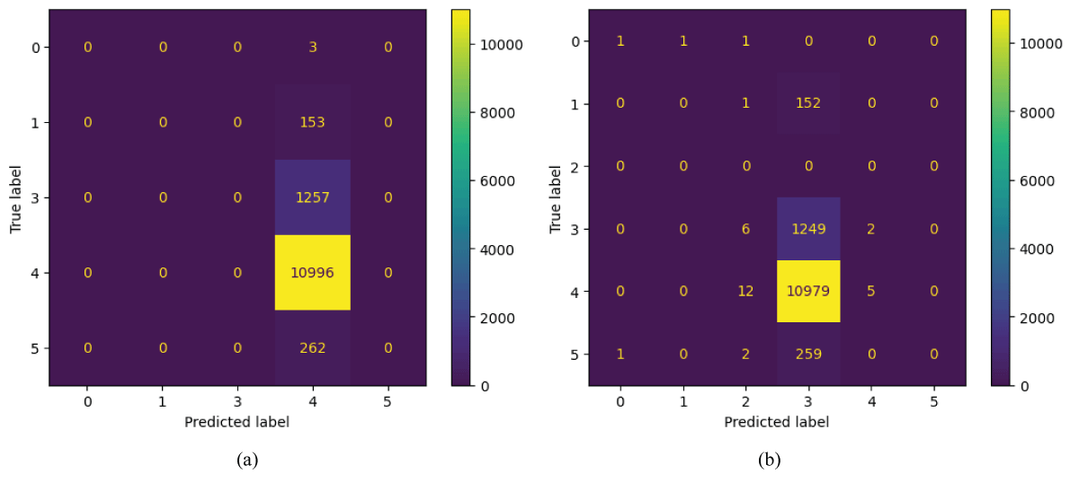
Figure 5 (a) shows the confusion matrix of the 1D-CNN model for audio signal classification. The Class 4 has 10996 correctly classified samples, whereas the remaining classes have fewer misclassified samples, i.e., 3, 153, 1257, and 262 samples with respect to Class 4 [18-24]. The matrix indicates strong performance, with the majority of predictions concentrated along the diagonal. Three samples from Class 0, 153 samples from Class 1, 1257 samples from Class 3, and 262 samples from Class 5 were incorrectly classified with respect to Class 4. Overall, the 1D-CNN model demonstrates high accuracy and effective feature learning in classifying audio signals.

Figure 5 (b) shows the confusion matrix of the simple RNN model for audio signal classification [18-24]. The Class 3 has a lower number of samples correctly classified, i.e 1249, whereas Class 4 has a higher number of misclassifications with respect to Class 3, i.e 10,979 samples. Further, the remaining classes have fewer misclassifications with respect to Class 3 [18-24]. The matrix indicates that the model performs effectively, with most predictions correctly aligned along the diagonal. Only a few misclassifications occurred, such as 6 samples from class 3, 12 samples from class 4, and 2 samples from Class 5 being incorrectly predicted with respect to Class 2. Overall, the Simple RNN model shows good classification performance with minor errors across a few classes.

Figure 5: Confusion Matrices of 1D-CNN and RNN models (a) 1D-CNN model confusion matrix (b) Confusion Matrix of RNN model .

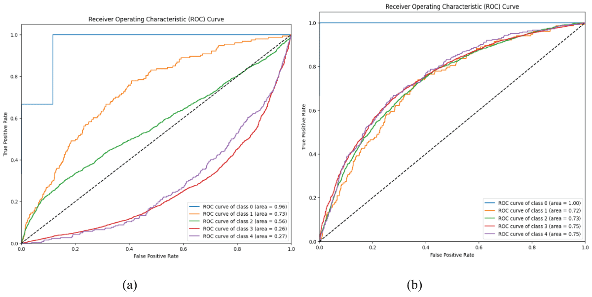
Figure 6 (a) presents the ROC curve for the 1D-CNN model, illustrating the trade-off between the pod and false positive rate across different classes. The 1D-CNN model has a higher AUC value of 0.96 for Class 0, whereas the remaining classes have lower AUC values of 0.73, 0.56, 0.26, and 0.27 for the remaining classes [18-24]. The Area under the Curve (AUC) values indicate that class 0 achieves the best performance with an AUC of 0.96, followed by class 1 with 0.73, and class 2 with 0.56. In contrast, class 3 and class 4 show relatively lower AUC values of 0.26 and 0.27, respectively. Overall, the 1D-CNN model demonstrates strong discriminative ability for certain classes, reflecting effective feature extraction and classification performance.

Figure 6 (b) shows the ROC curve of the simple RNN model. The RNN model has an excellent AUC value of 1.00 for Class 0 and lower AUC values of 0.72, 0.73, 0.75, and 0.75 for Classes 1 to 4, respectively [18-24]. The ROC curve indicates that the model achieves strong discriminative performance, particularly for class 0, which attains an AUC of 1.00, representing excellent classification. Other classes, such as class 3 and class 4, also perform reasonably well with AUC values around 0.75, while classes 1 and 2 have slightly lower AUCs of 0.72 and 0.73, respectively. Overall, the RNN model demonstrates reliable classification capability, with class 0 showing near-perfect separation performance.

Figure 6: ROC curves of 1D-CNN and RNN models (a) ROC curve of 1D-CNN model (b) ROC curve of RNN model.

Conclusion

The present work demonstrates audio signal classification using deep learning networks such as 1D-CNN and RNN models. The 1D-CNN has higher accuracy, i.e 86.77% compared to the simple RNN model. The 1D-CNN has a higher number of samples correctly classified for Class 4 compared to other classes. The simple RNN model has a lower number of samples correctly classified for Class 3 compared to other classes. Both 1D CNN and RNN models have higher AUC values for Class 0 compared to the remaining classes. Therefore, it can be said that the 1D CNN and RNN models have good classification performance for the audio dataset. These findings confirm that CNN-based architectures are more efficient for audio classification tasks compared to traditional sequential models. Further in the future, the 1D-CNN and RNN models have potential applications in real-time speech emotion recognition, environmental sound monitoring, and multimedia content analysis.

References

1. Hershey S, Chaudhuri S, Ellis DP, Gemmeke JF, Jansen A, Moore RC, Plakal M, Platt D, Saurous RA, Seybold B, Slaney M. CNN architectures for large-scale audio classification. In: 2017 IEEE Int Conf Acoust Speech Signal Process (ICASSP). 2017 Mar; p. 131‑135.

2. Choi K, Fazekas G, Sandler M, Cho K. Convolutional recurrent neural networks for music classification. In: 2017 IEEE Int Conf Acoust Speech Signal Process (ICASSP). 2017 Mar; p. 2392‑2396.

3. Kumar R, Gupta M, Ahmed S, Alhumam A, Aggarwal T. Intelligent audio signal processing for detecting rainforest species using deep learning. Intell Autom Soft Comput. 2022;31(2):692‑706.

4. Gupta M, Sharma R. Deep learning‑based environmental sound classification using CNN and RNN architectures. J Intell Syst. 2021;30(4):415‑427.

5. Pons J, Lidy T, Serra X. Experimenting with musically motivated convolutional neural networks. In: Proc 14th Int Workshop Content‑Based Multimedia Indexing (CBMI). 2016 Jun; p. 1‑6.

6. Zaman K, Sah M, Direkoglu C, Unoki M. A survey of audio classification using deep learning. IEEE Access. 2023 Oct;11:106621‑106652. doi:10.1109/ACCESS.2023.3318015.

7. Bhangale P, Kothandaraman R. Deep learning architectures for audio classification: A comparative study of CNN and RNN models. Int J Eng Res Technol (IJERT). 2020;9(8):123‑130.

8. Qamhan MA, Altaheri H, Meftah AH, Muhammad G, Alotaibi YA. Digital audio forensics: microphone and environment classification using deep learning. IEEE Access. 2021;9:62719‑62733.

9. Kumar R, Gupta M, Ahmed S, Alhumam A, Aggarwal T. Intelligent audio signal processing for detecting rainforest species using deep learning. Intell Autom Soft Comput. 2022;31(2):693‑706. doi:10.32604/iasc.2022.019811.

10. Aslam MA, Sarwar MU, Hanif MK, Talib R, Khalid U. Acoustic classification using deep learning. Int J Adv Comput Sci Appl (IJACSA). 2018;9(8):153‑159.

11. Purwins H, Li B, Virtanen T, Schlüter J, Chang S‑Y, Sainath T. Deep learning for audio signal processing. IEEE J Sel Top Signal Process. 2019 May;13(2):206‑219. doi:10.1109/JSTSP.2019.2908700.

12. Akinpelu, Viriri S. Deep learning framework for speech emotion classification. IEEE Access. 2024 Oct;12:152152‑152182. doi:10.1109/ACCESS.2024.3474553.

13. Hashemi M, Aghabozorgi M, Sadeghi MT. Persian music source separation in audio‑visual data using deep learning. In: Proc 6th Iranian Conf Signal Process Intell Syst (ICSPIS). Yazd, Iran. 2020 Dec; p. 1‑6. doi:10.1109/ICSPIS51611.2020.9349614.

14. Hasan H, Rahman MSM, Islam MS. Audio forensic authentication using background noise. Appl Intell. 2015 Mar;42(3):627‑641. doi:10.1007/s10489‑014‑0629‑7.

15. Hassan E, Elbedwehy S, Shams MY, Abd El‑Hafeez T, El‑Rashidy N. Optimizing poultry audio signal classification with deep learning and burn layer fusion. J Big Data. 2024 Sep;11(135):1‑29. doi:10.1186/s40537‑024‑00985‑8.

16. Alzahrani MA, Aljohani M, Alzahrani MA. Audio‑based activities recognition using machine learning algorithms and deep learning. Sensors. 2019 Oct;19(4819):1‑19. doi:10.3390/s19224819.

17. Kim JW, Salamon J, Li P, Bello JP. Crepe: A convolutional representation for pitch estimation. In: 2018 IEEE Int Conf Acoust Speech Signal Process (ICASSP). 2018 Apr; p. 161‑165.

18. Reddy BL, Uma Mahesh RN, Nelleri A. Deep convolutional neural network for three‑dimensional object classification using off‑axis digital Fresnel holography. J Mod Opt. 2022;69(13):705‑717. doi:10.1080/09500340.2022.2081371.

19. Mahesh RN U, Nelleri A. Multi‑class classification and multi‑output regression of three‑dimensional objects using artificial intelligence applied to digital holographic information. Sensors. 2023;23:1095. doi:10.3390/s23031095.

20. Uma Mahesh RN, Lokesh Reddy B, Nelleri A. Deep learning‑based multi‑class 3D objects classification using digital holographic complex images. In: Sivasubramanian A, Shastry PN, Hong PC, eds. Futuristic Communication and Network Technologies. VICFCNT 2020. Lect Notes Electr Eng. Vol 792. Springer, Singapore; 2022. p. 43. doi:10.1007/978‑981‑16‑4625‑6_43.

21. Uma Mahesh RN, Basavaraju L. Three‑dimensional (3‑D) objects classification by means of phase‑only digital holographic information using Alex Network. In: 2024 Int Conf Signal Process Comput Electron Power Telecommun (IConSCEPT). Karaikal, India. 2024; p. 1‑5. doi:10.1109/IConSCEPT61884.2024.10627906.

22. Uma Mahesh RN, Basavaraju L. Deep learning‑based multi‑class three‑dimensional (3‑D) object classification using phase‑only digital holographic information. IgMin Res. 2024 Jul 9;2(7):550‑557. doi:10.61927/igmin216. Available from: igmin.link/p216.

23. Mahesh RU, Nagaraju S. Three‑dimensional (3‑D) objects classification by means of phase‑only digital holographic information using deep learning. In: Data Science & Exploration in Artificial Intelligence: Proc 1st Int Conf Data Sci Exploration Artif Intell (CODE‑AI 2024). Bangalore, India. 2024 Jul 3‑4; Vol 1. CRC Press; 2025 Feb. p. 363. doi:10.1201/9781003587392‑53.

24. Uma Mahesh RN, Rajanahalli Nataraj, Puttaswamy C. Deep residual network for three‑dimensional (3‑D) objects classification using phase‑only digital holographic information. J Intell Syst. 2026;35(1):20240393. doi:10.1515/jisys‑2024‑0393.

About the Article

Cite this Article

RN Uma Mahesh , Chakrasali D, N Suhas Chandra Thejasvi , C Manoj Kumar , Bharadwaj SD. Audio Signal Classification Using Deep Learning. IgMin Res. June 19, 2026; 4(6): 208-214. IgMin ID: igmin345; DOI:10.61927/igmin345; Available at: igmin.link/p345

• DOI10.61927/igmin345

06 Jun, 2026

Received

18 Jun, 2026

Accepted

19 Jun, 2026

Published

Share this Article

Anyone you share the following link with will be able to read this content:

Get shareable link

Topics

Artificial Intelligence