IGMIN: We're glad you're here. Please click 'create a new query' if you are a new visitor to our website and need further information from us.
If you are already a member of our network and need to keep track of any developments regarding a question you have already submitted, click 'take me to my Query.'
Welcome to IgMin Research – an Open Access journal uniting Biology, Medicine, and Engineering. We’re dedicated to advancing global knowledge and fostering collaboration across scientific fields.
At IgMin Research, we bridge the frontiers of Biology, Medicine, and Engineering to foster interdisciplinary innovation. Our expanded scope now embraces a wide spectrum of scientific disciplines, empowering global researchers to explore, contribute, and collaborate through open access.
Welcome to IgMin, a leading platform dedicated to enhancing knowledge dissemination and professional growth across multiple fields of science, technology, and the humanities. We believe in the power of open access, collaboration, and innovation. Our goal is to provide individuals and organizations with the tools they need to succeed in the global knowledge economy.
IgMin Publications Inc., Suite 102, West Hartford, CT - 06110, USA
The advent of room- temperature superconductors in electrical, electronic and super computing platforms, has been a dream since long time. This dream can only come true by understanding the origin of superconductivity in all superconductors. In this paper, the origin of the attractive interaction between electron pairs in superconductors are discussed, with emphasis on the role of neutrons and their direct relation to the isotope effect. Amazingly enough, no one has tried to investigate the true role of neutrons and its contribution to the superconductivity phenomenon, since its discovery in 1911. Indeed, all previous theories including the extensions of the Bardeen-Cooper-Schrieffer (BCS) theory, failed to explain the common origin of superconductivity in all types of superconductors. In this paper it is proposed that the system of electrons and nucleons (neutrons in particular) can form bosons, which may form a condensate of superconducting pairons. In the proposed theory, the hyperfine interactions (HFI) between electrons and surrounding nucleons result in pairon charge neutralization that transform some electron pairs into pairons at low temperature. We analyze the role of neutrons (which consist of charged quarks) in coupling some mobile electrons (or holes) in all types of superconductors at sufficiently low temperature. We also review some existing experimental results, which we consider as evidence supporting the proposed theory. These experiments were carried out for other investigation purposes about the properties of superconductors and their applications (e.g., in nuclear magnetic resonance NMR and fission nuclear reactors).In spite of the theoretical nature of this work, the proposed new theory is supported by some evident observables such as the Isotope Effect in superconductors, which is strongly related to the neutron content in the superconductor.
Until now, the superconductivity has not been completely understood, as agreed upon by the majority of researchers in this field [1-10,59,83]. Many researchers proposed interesting explanations of the phenomenon. Among these one can distinguish the Ginzburg-Landau (G-L) macroscopic theory [1]. The progress in understanding superconductivity gained a great momentum in the mid-1950s, by the Bardeen-Cooper-Schrieffer (BCS) theory [2]. According to the BCS theory, the current is carried in superconductor by pairs of electrons known as Cooper pairs (pairons). Therefore, the Cooper-pair should be formed by electrons with opposite spins (s=±½) and opposite wavevectors (±k) at the Fermi surface. The coupling between such pairs is carried out (supposedly, via phonons) for a small fraction of the electrons. In conventional superconductors, this attraction is usually referred to as the electro-phonon interaction [3]. The BCS theory predicts that the lowest energy state of super-conducting pairs is separated from higher energy states of unpaired electrons by an energy gap, which prevents any energy loss of electron transport at low temperatures. The electron pairs have a slightly lower energy and leave an energy gap above them on the order of 1 meV. In fact, the BCS theory predicts a band gap (Eg= 2∆) of 7/2 kBTc. Which results in a maximum Tc = 23.3K.Nevertheless, after the discovery of High-Tc superconductor (HTS) materials with Tc>30K in the late 1980s, it was believed that BCS theory alone cannot explain the super-conductivity phenomenon in all superconductors and that other effects are in play [59]. The subsequent theories, which were proposed to explain superconductivity in HTS materials, are enormous [4-10, 54-59]. For instance, the Anderson resonating-valence-bond (RVB) theory is based on the coupling role of singlet spin pairs [4]. According to the RVB theory, the singlet magnetic pairs become Cooper pairs when the parent insulator is sufficiently doped. Later, the whole theory of superconductors assumed that superconductivity mainly occurs due to pairing of hole carriers [5]. Other theories assumed the existence of charge stripes between the 2D layers of superconductors which play the coupling role between pairons [6].
In this paper we summarize the state-of-the-art in superconductivity modeling approaches, and describe the proposed theory of superconductivity in all superconductors. The paper is organized as follows. The next section is dedicated to discussion on the origin of attractive interaction in superconductors. In this section, I explain the broad lines of my neutron-pairon coupling model. In the following section, I present the mathematical modeling procedure. Subsequently, we present some simplified solutions of the proposed model. Finally, I demonstrate the validity of my theory and present my conclusions.
Origin of attractive interaction in superconductors
Until now, the mechanism by which two negatively charged electrons are tied together to make a pairon in a superconductor is not fully understood [39,58,59,73,79]. The origin of this interaction is still a controversial topic, especially in HTS materials. In the BCS, phonons are assumed as the mediators making the attractive interaction between pairs of electrons in superconductors. Other BCS-like models, replace the role of phonons by other quasiparticles, such as, plasmons [7], excitons [8], polarons [9] and magnons [10]. All of these suggestions have their reasoning, but we always return to the first question: How are similar charge carriers (electrons!) are actually paired? In order to find an answer we propose the role of nucleons, and neutrons in particular, through their hyperfine and dipole interactions.
In the following subsections we describe to important observable phenomena, which support our theory. These phenomena are all about the electron neutron dipole moments and the hyperfine interactions.
Neutron-electron interactions
The neutron has a half spin and an intrinsic magnetic dipole moment, so that it is influenced by external electromagnetic fields. The magnetic moment of a neutron (due its spin) is negative (µn ≈ -1.913 µN), where µN = eh/2mp is the nuclear magneton and mp is the proton mass. Neutron magnetic moment is negative because its orientation is opposite to its spin. Neutron spin is polarized upon transmission through a magnetic field. The repulsion force between neutrons and external magnetic field depends on the field strength (B) and the magnetic moment of neutrons (µn). In fact this repulsion energy (µnB) is a part of the neutron potential [11]. A magnetic moment is a vector, and its direction is defined by the neutron spin (µn= µns). The exerted torque by an external magnetic field on a neutron aligns the neutron spin vector opposite to the magnetic field. The neutron has also an electric dipole moment (nEDM) due to the distribution of positive and negative charge inside it. Although electrically neutral, the neutron is made up of charged quarks. An imbalance of neutron charge (offset between the centers of positive and negative charge) can therefore cause a non-zero nEDM [12]. Although its existence violates the charge parity and time reversal principles, the nEDM is already anticipated in the Standard Model (SM) of particles and Supersymmetry theory (SUSY) in nuclear physics [13]. Figure 1 summarizes the neutron–electron interactions outside the nuclei of a solid. As shown in the figure, the electromagnetic interaction is described by the Quantum Electrodynamics (QED). Also, the quantum nonlocal effects influence both nucleons and electrons. For more details about the neutron nonlocal quantum effects and how they can be modeled (Fermi pseudo potential), refer to Li, Potel & Nunes [14].
Figure 1: Schematic diagram of the mechanisms of neutron-electron interactions of electromagnetic origin. QED stands for Quantum electrodynamics and QFD stands for Quantum Flavor dynamics. More details about QED and QFD can be found in [14].
Neutron Hyperfine Interactions (HFI)
The neutron hyperfine interaction is just like the other nucleons hyperfine interactions due to magnetic (spin) coupling, between the nucleon and surrounding electrons. Here, we just consider the specific physical parameters of neutrons. Generally speaking, the nucleon-electron interactions are based on both magnetic and electrical dipole moments of both electrons and nucleon. In fact, the experimental investigations suggest that the magnetic dipole (spin) and charge degrees of freedom are highly entangled in superconductors [15]. The spin polarization can transfer from electrons to nuclei constituents (protons and neutrons), and thereby aligning the nuclear spins according to the electron spins at a given magnetic field. This process is called the dynamic nuclear polarization (DNP) [16]. This happens when electron spin polarization deviates from its thermal equilibrium value, and the polarization transfers between electrons and nuclei can occur spontaneously via the electron-nuclei hyperfine interaction (HFI) [17]. Generally speaking, the HFI may be classic (dipole-dipole) interaction or quantum (Fermi-contact). The quantum contribution happens when an electron is found right on top of a nucleon spin, Therefore, they interact via the so-called Fermi-contact potential or quantum HFI [18]. This part is symmetric, and given by the following expression (normalized by ℏ)(1):
where µo is the magnetic permeability, µB is the Bohr magneton, µn is the nuclons magneton, gn and ge are the g-factors (of nuclons and electrons, respectively)(2) and |ψ(0)|2 is the electron wave probability density function. Otherwise, when the electron wavefunction has an angular dependence (e.g., p-, d-, f-orbitals), then neutrons and electrons can also interact through the dipole-dipole interactions (the classical, part of HFI). The dipole-dipole interactions are, in general, angle dependent and anisotropic. This is likely to happen in transition metals and low-dimensional structures (e.g., cuprate superconductors). The interaction energy of such electrons and nearby neutrons, is given by:
(1)The g-factor or dimensionless magnetic moment is a proportionality constant that relates the observed magnetic moment μ of a particle to its spin angular momentum quantum number (S): μ = g(e/2m)S. To make it dimensionless, it is scaled by a unit of magnetic moment, usually the Bohr magneton (µB = eℏ/2me) or nuclear magneton (µN = eℏ/2mp). Recent experiments yield ge ≈ 2.002319 [84]. The so-called magnetic anomaly of electrons ae = (ge −2)/2, is the relative deviation of the electron magnetic g-factor from the Dirac value 2. The so-called Lande factor is the total angular momentum g-factor from both spin and orbital angular momentum of an electron, J = L + S.
where θ is the angle between a neutron dipole and an electron dipole (e.g. the p-orbital lobe) and r is the average distance between them, as shown in Figure 2. In general, both isotropic and anisotropic HFI (As and Ap) can exist, depending on the material crystalline structure. Therefore, the HFI sum is given by:
Figure 2: Schematic of neutron-electron hyperfine interactions, showing how the neutron dipole moment interacts with isotropic s-orbitals and anisotropic p-orbital lobes. Here, Bo is the external magnetic field, while Bn and Be are local magnetic fields of neutrons and electrons.
(3)
In solid materials, the nuclear site symmetry is important. For cubic lattices, only the symmetric part As component is important. Otherwise, the HFI can be represented as a 2nd order tensor A[3x3], as follows:
(4)
Here, the rotation angles Θ and Φ are between the diagonalized tensor axes X,Y,Z and the adopted system axes. The above equations only consider the local coupling interactions between nuclear spins and the surrounding electrons of the same site. However, the RKKY (Ruderman-Kittel-Kasuya-Yosida) interaction shows that electrons on a given site can interact as well with neighbor sites [19]. Therefore, the HFI can transfer between the local moment and the nearby nuclei spins [20]. In order to consider the transfer of HFI coupling across neighbor nuclei, we can express A as an expansion:
(5)
where Ao is the intrinsic HFI coupling constant of the considered nucleous site and Ai is the contribution of neighbor sites at distance r. Also, q is the wavevector of the HFI coupling transfer. This phenomenon justifies my ansatz of the propagation of the neutron polarization waves in the crystal lattice of a superconductor (Figure 2).
How are neutrons polarized in a crystal lattice?
Neutrons can be polarized by nature forces, such as electromagnetic (~300 neV/T), strong nuclear (~100 nV), weak nuclear (10-7 of polarization by strong forces) and gravity (very small, 100 neV/m). In addition, the HFI, due to electrons-nuclei quantum interaction), can polarize the neutrons inside nuclei [14]. Noteworthy, the neutron polarization can be induced (or increased) by the hydrostatic pressure, due to change of inter-atomic distances. Finally, it should be noted that polarization can happen in different directions and can move and transfer from atom to another, in conjunction with carrier transport.
How do superconductors superconduct?
Now we come to outline the proposed theory of superconductivity. Due to the experimentally-verified observables, that we discussed above,we believe in the role of nucleons in general and neutrons in particular, as the origin of superconductivity at low temperature [83]. As neutrons are composed of both negative and positive quarks, they have a long range electromagnetic effect on both electrons and holes in superconductors [21]. The neutron moments interact with mobile carriers through HFI [17,18]. The arrangement of nucleon spins in response to surrounding electrons polarities is well known in physics, and sometimes called the dynamic nuclear polarization [21]. The HFI couples some pairs of electrons (which are arranged in specific configurations, as explained in the next section) and propagate across the crystal lattice sites. When coupled pairs of electrons (preformed pairons) are exactly tuned (have same wave vector and group velocity) like neutron polarization waves they can condense in a single ground-state. This tuning condition of preformed pairons can only happen below a specific critical (Tc). Otherwise, superconductivity will not appear or may only happen temporarily as short decaying packets (beating, when the two waves are not exactly tuned). The ground-state pairons can hence propagate, with their HFI coupling interaction like a single coherent wave.
Neutron-pairon coupling model
The neutron coupling can only happen to a number of mobile charges (conduction electrons or valence holes) when their spins and momenta are properly aligned with neutron dipole moments. Neutrons may couple with even numbers of mobile charge carriers (pairons, bi-pairons, tri-pairons, etc). Therefore, three neutrons can couple one pairon of conduction electrons (or valence holes), if their direction of motion and spin are aligned in certain configurations. Figure 3 depicts one of the possible electron-neutron interaction configurations. Of course other scenarios are possible with less or more coupling strength(3).
(3)It is well known from nuclear physics that nucleons (neutrons and protons) can pair and cluster under the effect of strong nuclear forces and the pairing process is influenced by the so-called 3N forces [21]. However, the coupling neutrons, in the proposed model, are most likely belonging to different atoms of the superconductor.
Figure 3: Schematic illustration of a possible configuration of the electron-neutron interaction mechanism. The three neutrons are most likely from different atoms. Note that neutrons have a huge number of quarks and antiquarks, which are continuously generated and annihilated. Only the three valence (upper-shell) quarks of the neutron are shown here (1 up quark, termed u, and 2 down quarks, termed d).
As shown in Figure 3, coupling may happen when two interacting electrons of opposite spin (singlet state)(4) are aligned between three polarized neutrons. This means that the three neutrons have their spins aligned to have a total charge unbalance of ±2e (total up- and down-quarks each of charge: ±2e/3) in this minimal con-figuration. Similarly, pairons of missing electrons or valence holes (with charge +2e) can go through subsequent attraction and repulsion with 3 neutrons (with up- and down-quarks of charge: ±2e). The subsequent attraction and repulsion of pairs will minimize their energy and inhibit any collision (or net exchange of energy) between them and the nearby atoms. The pairon interaction becomes maximal (resonant) when the pairon-neutron dipoles are aligned at certain angles and therefore, paired electrons wave-vectors are completely de-phased. This mechanism can happen, not only in the bulk of simple elemental superconductors, but also in localized regions of layered HTS compounds.
(4)This does not mean that electrons with triplet, or generally multiplet, spin states are excluded in our theory. The Pauli condition for a particle or composite particle (of two or more particles) to have Bosonic behavior is to have an integer total spin value (S = 0, 1, 2,..). Therefore singlet pairs (with S=0) as well as triplet pairs (with S=1) can form pairons.
Any successful quantum theory about superconductivity should have a clear physical side (physical model) and a mathematical representation side (mathematical model). Indeed, superconductivity is essentially a macroscopic quantum phenomenon. However, the proposed theory can be analyzed by a variety of macroscopic and microscopic methods. The microscopic description of superconductivity needs a many-body quantum approach. In such microscopic quantum approaches, the main task is to find the eigenvalues (energies) and eigenvectors (wave functions) of the system Hamiltonian. In the proposed model, we consider both nucleons (inside their nuclei) and the surrounding electrons. However, we’ll see that we end up with a system of electrons (part of them is paired) and their correlations and interactions with the solid nuclei. Considering valence holes, beside conduction electrons, means that we need to consider the whole effective system of electrons(5).
(5)The mathematical treatment of holes is much easier than treating with the whole number of valence electrons. This is clear when we have a solid with distinct (non overlapped) conduction and valence bands.
The Hamiltonian of the superconductor system is composed of an intrinsic part Ho due parent material host atoms, an extrinsic part Ho2, due to doping and/or impurity atoms, and an external-field dependent part Hext:
(6)
The intrinsic Hamiltonian, Ho, can be subdivided into three components:
(7)
with
(8a)
(8b)
(8c)
where the subscript e(h) stands for electrons (holes) and n(p) stands for neutrons (protons), or generally nucleons. The first term H1 sums up the kinetic energy of unpaired charge carriers (He and Hh). These are conduction electrons and valence holes. For electrons, the kinetic energy (Ek = p2/2me = 2k2/2me) is measured above the Fermi energy EF in metals or the conduction band edge Ec in non-metallic materials. Also, the kinetic energy of holes (Ek = p2/2mh = 2k2/2mh) is measured below the valence band edge in non-metallic materials. The interaction with external electromagnetic fields, with a vector potential A, and/or a scalar potential φ, can be also considered here (instead of Hext). For instance, the potential momentum eA can be added to the kinetic momentum p=ћk of unpaired electrons in He. This allows simulating the de-pairing effect, when an applied external magnetic field exceeds a certain critical value. Note that we can exclude the kinetic self energies of nucleons (which are almost static), with respect to electrons. Therefore, both Hn and Hp can be neglected, unless we want to study the role of lattice vibrations (phonons).
The second term H2 includes the Columbic correlations of electrons and holes with themselves, as well as all possible scattering and recombination/geneatin mechanisms. This is typically termed as U in the literature. The electron-proton interaction (He-p) can be considered in the Columbic term, although the proton charge is typically screened from outer conduction electrons, by the tightly-bound core electrons(6). On the other hand, the strong and weak nuclear interactions between nucleons are short-range (inside their respective nuclei), except for some nonlocal quantum interactions [21]. Also, the nuclear electromagnetic interactions are long range but much smaller (between nucleons of different nuclei) than their interactions with electrons (because of the large mass ratio of nucleon/electron). Therefore, the nucleon-nucleon interactions Hn-n may be neglected in our superconductor system.
The most important interaction term in a superconductor is obviously the coupling term, H3, of pairons (or multi-pairons). This term is mainly due to electromagnetic dipole-dipole interactions as well as the quantum HFI interaction between nucleons and paired electrons. This term can be described by the following equations.
(9)
Generally speaking, the spin term originates from HFI and mixes the electron and the nuclear-spin states and can form composite spin multiplets. Actually, the total HFI between a nucleon, having a nuclear spin I, with an electron of spin S and momentum L at a distance r from the nucleus site can be calculated as a function of distance as follows [22]:
(10)
where γn = gnµN/ћ and γe = geµB /ћ are the gyromagnetic ratios of nucleons and electrons, respectively. The HFI is null for filled shells of electrons, as they have zero total spin (S) and zero total orbital angular momentum (L). Therefore, the spin part may be given as follows:
(11)
Here Aij is the HFI coupling tensor, which is given by equation (4) and can be calculated by ab-initio quantum simulation methods(7) [23] or measured by nuclear magnetic resonance (NMR) techniques [24]. Also, the electric multipole part (dipoles, quadripoles, etc) is due to charge inhomogeneities (of both electrons and nucleons, particularly of neutrons) and given by:
(7)The symmetric part of the hyperfine tensor [A] is usually calculated by the tight-binding (TB) method with augmented plane waves (APW) and the anisotropic part can be calculated by the pseudopotential method. These are actually empirical quantum methods, sometimes used in conjunction with density functonal theory (DFT) or nnonequilibrium Green’s functions (NEGF) ab-initio methods, and hence called semi-empirical quantum methods [25].
In fact, all the nuclei with spin I >½ are characterized by a non spherical nuclear charge distribution. These nuclei thus posses an electric quadrupole moment eQ ≠0 while their electric dipole moment is zero. However, the first term in the above equation, H(nEDM), is due to neutron charge imbalance(8). The second term is due to electric quadrupole interactions, which is extremely sensitive to the local charge symmetry. This term is proportional to the electric field gradient generated by the electronic charge distribution surrounding the nucleus. The Hamiltonian H(Q) can be written in terms of the quadropole moment Q and the field gradient tensor V, when it is diagonalized, as follows [26]:
(8)Although electrically neutral, the neutron is made up of charged quarks. An imbalance of charge of quarks will cause a non-zero neutron electric dipole moment (nEDM). The nEDM is believed to exist at some level to explain the matter-antimatter asymmetry of the Universe, although this would be a violation of parity and time reversal symmetries [12,13].
This can be also written in terms of the nuclear spin I, as follows:
(13b)
where Iz is the nuclear spin along the principle axis (Z-axis), I2=Ix2+Iy2+Iz2, (Vyy-Vxx)/Vzz is an asymmetry parameter and Ao is given by:
(13c)
where α is a constant. Noteworthy, the quadopole moment Q disappears in cubic and spherically symmetric charge distributions (e.g., due to s-electrons). Also, Q is null when I = ½ or I = 1, therefore the nuclear spin should be greater than one (I>1) for non-vanishing quadruple moment. The quadruple moment parameters can be obtained front nuclear quadruple moment resonance (NQR) experiments [27]. Finally, the electric dipole interactions, between neutrons and electrons, may be expressed like the London interaction, as follows [26]:
(14)
where dn and de are neutron and electron dipole moments, and r is the average separation between them. Also, r1, θ1 and r2, θ2 are the displacements and angles formed by the two dipoles with respect to the line connecting their centers. In addition, θ is the angle between them. Note worthy, the charge in-homogeneities, which stand behind the electric multi-pole term, have been identified experimentally by NQR [26] and NMR [27]. Figure 4 summarizes the electron-nucleon interactions outside the nuclei in a crystal lattice, which contribute in the superconductor Hamiltonian.
Figure 4: Summary of the electron-nucleon interactions outside the nuclei in a crystal lattice, which contribute to the superconductor Hamiltonian. Here, HFI stands for hyperfine interaction, nEDM stands for neutron electric dipole moment, and NQR stands for neutron quadratic resonance.
The correlative U term in the proposed model includes other types of intra ion-ion interactions, such as intra p-p, interactions. Actually, Tranquada and his collaborators reported the first observation of the splitting of spin and charge order peaks in cuprate superconductors by elastic neutron scattering [28].
Note that the heavy elements have about one and half as many neutrons as protons in the nucleus (N/Z ≈1.5), while mid-range elements have about one and a third (4/3) as many neutrons as protons in their nuclei. Generally, we can consider both neutron and proton magnetic moments via an effective gyrometric ratio, taking into account that µn/µp = -0.68497935.
The role of impurities may be considered, implicitly, as part of the superconductor unit cells (or super-cells). However, the impurity atoms have local potentials and interactions, which are different from host atoms. Also, intentionally doped impurities may form impurity bands inside the energy gap of highly-doped insulating materials. Therefore, we should better consider an additional impurity Hamiltonian (Ho2), which may take the same inclusive form of that of host atoms, such that:
(15)
The Columbic interactions of impurities with surrounding electrons and other charge carriers (H2’) resembles the corresponding Hartree-Foch term in the Hamiltonian of host atoms (H2), with a suitable screening potential. Also the participation of impurities in pairon coupling (H3’) resembles the corresponding coupling term in the Hamiltonian of host atoms (H3), with no duplication of their nuclei sites. Neglecting the kinetic energy of fixed impurities, the impurity Hamiltonian may take the following simple form:
According to Korshunov, Togushova and. Dolgov, this Hamiltonian may be written as follows [29]:
(16b)
Here, the first term (H2’) represents the Columbic (electrical) interaction of impurities and the second term (H3’) represents the spin (magnetic) interactions, which are important for magnetic impurities. Note that in most cases only a few near-neighbor shells of the impurity should be considered. Of course, we should consider the specific features of impurities, such as their screened Columbic potential (U) and their spin coupling (J) and hence the HFI with surrounding electrons. Fortunately, the NMR can help a lot to probe such effects [22]. Therefore, the impact of impurities can be incorporated into the HFI coefficients of the coupling term of the proposed model. Figure 4 shows the electron-nucleon interaction outside the nuclei of a crystal lattice, which contribute in the superconductor Hamiltonian
The mathematical modeling and solution procedure may start with a simple Hamiltonian containing all kinetic energies of mobile charge carriers (electrons and/or holes), as well as the interaction potentials, including the pairon coupling term. For simplicity, the Hamiltonian of a single-band system of mobile electrons and neutron-coupled pairons (of 2 electrons) will be considered here. Therefore, the system Hamiltonian can be written, in a second quantization form (using field operators), as follows:
(17)
Here, the indices k, K and L combine the wavevector and spin of electrons, coupled pairons and polarized coupling neutrons (which I call n-polarons), respectively. Also, Ek is the kinetic energy of normal Bloch electrons (Ek = ћ2k2/2mn) measured from Fermi level. nk is the electron number operator (nk = ak†ak with ak† and ak are the electron creation and annihilation operators). In addition, nK and NL are the number operators of coupled (preformed) pairons and their coupling polarons, respectively. Finally, DKL represents their coupling strength between them. Note that we can use groups of paired electrons and n-polarons (e.g., 2 paired electrons and 3 n-polarons) such that nK = nk1 nk2 and NL = Nl1.Nl2,Nl3. Therefore, nki nk2 are the number operator of paired electrons and Nl is the number operator of surrounding n-polarons which couple them (Nl = c†l cl with c†l and cl are the creation and annihilation operators of polarized neutrons). Note that I use the new term ‘n-polarons’ to refer to the quasi-particles, associated with the neutron polarization waves, to distinguish them from the conventional polaron quasiparticles, which are well known in solid-state physics [30]. The first term in the above Hamiltonian of (17) corresponds to the normal state of electrons. The second term includes the Columbic interactions between charge carriers (electrons with them-selves and core ions, for such a one-band system). Therefore, a suitable screening potential (Vckk') should be considered, such as the Fukagawa potential (V(r) ~ (1/r).exp(-r/λ), where λ is the screening length).
The third term corresponds to the nucleon-electron interaction energy, with emphasis on the role of neutron-electron interactions. This term is responsible for superconductivity in the present theory. In order to properly evaluate the coupling term, the spin and momentum of paired electrons should be matched with polarized neutrons, and the quantum coupling between them should be considered in terms of the HFI potential. Actually, both neutrons and protons participate in the HFI, through their spins and magnetic moments. However, protons are strongly screened by core electrons and their screened electrical interaction with conduction electrons is clear in Figure 5. This figure shows an idealized potential wells of nucleons (protons and neutrons). However, the role of neutrons is more significant because of their dominant number (N/Z~3/2). Also, the neutron electrical dipole moment (nEDM) is thought to play an equal footing mediating role for both electron-pairing and hole-pairing, as discussed above.
Figure 5: Schematic of idealized potential wells of nucleons (protons and neutrons) inside a nucleus. Note that n stands for neutrons and p stands for protons.
In all cases, we can simplify the coupling term, and hence the superconductor Hamiltonian, by establishing a relation between the number operators of polarized neutrons and pairons. For instance, we can assume the number of polarized neutrons per pairon N/ns=3, just like the suggested coupling configuration, or expand N ≈ α+β.ns, where α and β are constants and ns is pairon density. Then, we can substitute the number operator (NL) and reduce the coupling term as follows:
(18)
where the expansion coefficients αL and βL are constant operators, which refer to the intrinsic site-dependent HFI and the propagating part of polarized neutrons. These coefficients resemble the α and β parameters in the G-L theory of superconductivity, which represent the expansion coefficients of the condensation energy in terms of the pairon density (ns). Therefore, the present model gives an additional physical background to the phenomenological G-L theory [1]. In the above form, the coupling term is a quadratic polynomial of pairons density.
Once the physical Hamiltonian of the superconducting system is mathematically constructed, it should be diagonalized to find out its ground-state eigen-energies (i.e., the energy band structure) as well as the excitation energies and hence the system properties. As the dimension of the occupation number space (Hilbert space) associated with such a quantum many-body system is large, it is a big challenge to solve the problem even with very powerful computers. Despite the fact that for the Hamiltonian matrix is sparse (99% of elements are zeroes) the dimension grows exponentially M = 22Ns, where Ns is the number of electron levels in the model. The exponential growth of basis size puts serious restriction on lattice size. Therefore, the Hamiltonian should be reduced with a suitable approach, such as the mean-field approximation (MFA), where we keep only the first order perturbation terms [31]. Applying the MFA to the correlation (U) and pairing interaction term of the superconductor Hamiltonian leads to a reduced Hamiltonian, with Hartree-Fock (H-F) and pairing fields. However, the MFA should be applied with high attention, for strongly correlated systems. In fact, the MFA assumes that the influence volume of one particle (pairon) to contain the effect of many similar particles so that the interaction can be taken as the average of many pairons. In the BCS theory, this works well for LTS superconductors. However, in HTS materials, like cuprates, the number of pairons per unit volume is about one. Therefore, the MFA will not properly work for such materials. The dynamic mean-field theory (DMFT) may be rather utilized to treat strongly correlated systems [32]. In contrast to the MFA approaches, such as the self-consistent dynamic field theory (SC-DFT) [33], the mean-field in the DMFT is energy-dependent. Starting from band structure and local quantum interactions (e.g., around impurities), the DMFT approach maps the Hamiltonian onto a single-site model. The only approximation of the DMFT is the neglect of spatial fluctuations of the lattice self energy. This is acceptable for a lattice with infinitely large coordination, i.e., when the number of neighbors of each site is infinite. The so-called ‘Cluster DMFT’ is an improved extension of the DMFT to correlated clusters, for finite-dimensional systems [34]. Actually, both DMFT and Cluster DMFT have been used successfully with several Hubbard models, which are in generally intractable with conventional perturbation expansion techniques [35]. The numerical solution approaches include Lanczos diagonalization [36] of small clusters to density-matrix-renormalization-group (DMRG) studies of n-leg ladders [37] and quantum Monte Carlo simulations of two-dimensional lattices [38]. The quantum Monte Carlo (QMC) method is a universal tool for the numerical study of quantum many-body systems with strong correlations. The so-called determinstic QMC scheme has been already used for the numerical study of physical models with strong interactions, e.g., for HTS materials, [39].
Code implementation method
Because of the similarity of the mathematical structure of the proposed Hamiltonian and the Hubbard t-U-J model [40], we can start from one of the published codes, e.g., [41,42,83,85]. The complete listing of our code can be found in [83]. In particular, the reference [42] depict the exact diagonalization C++ library (EDLib) for solving quantum electron models, including the single-band finite Hubbard cluster and the multi-orbital impurity Anderson model. The observables that can be computed using EDLib are the single particle Green’s functions and spin–spin correlations [85].
We note that the spin operator in such block diagonal models has a similar form to the HFI coupling term in our theory. In fact, the t-U-J model has been utilized as a pairing Hamiltonian, to simulate High-Tc superconductors, with the J-term representing the pairing process by simple spin-singlets or spin triplets [43]. Also, the an-isotropic spin coupling terms as well as charge exchange terms have been considered within this model [44]. The latter model, with anisotropic spin-exchange interaction (t−U−J//−J⊥ model) and charge-exchange (pair hopping) interaction (t−U−I model), also known as Penson–Kolb–Hubbard model [45], are all sorts of extended Hubbard models (EHM). It should be noted that the HFI coefficients can be obtained from NMR measurements, as described in [22] or by ab-initio quantum methods. Also, the U correlation term cab be added, either separately (HEE = ΣiUi ni↑ ni↓, with Ui and ni are the Coulomb potential and the number operator of electrons on the ith site). For large repulsion, the model can be simplified into the t-J model, which explicitly contains an attractive interaction, inside the J coupling term, as explained in the Spalek paper [40].
In our code, the Lanczos algorithm [46] is utilized to diagonalize the Hamiltonian in an efficient manner. This algorithm iterates the vector W of eigenvalues, using the iteration equation: W W+H.v, starting from a basis vector |v0>. Actually, the Lanczos method does not require to complete the diagonalization process, enabling to obtain only a useful portion of eigenvalues of the system. The Lanczos algorithm can then help to find out the static and dynamic properties of the system. Therefore, the ground state calculations require the storage of 3 vectors of the size of the number of states. It is also known that the number of states scales exponentially with the size of the system. This limits the number of atomic sites to a few tens in the simulated lattice (on available hardware). There exist also multi-processing interfaces (MPI) such as OpenMP for parallelized versions of the finite temperature Lanczos diagonalization method to diagonalize Hamiltonian matrix and to compute observables [42]. I show a sample of results and some evidence proving the validity of the theory in the next section.
Application of mean-field approaches (MFA)
In MFA, the energy of charge correlations (U) as well as the pairon interaction energy are replaced by average quantities, which are physically meaningful. Therefore, the electronic correlations can be replaced by a Hartree potential, which can be iterated with Poisson’s equation to obtain a self-consistent solution. We add here some analysis concerning the pairon coupling term. In the context of MFT, we can keep only the first order perturbation terms of this term (DKL= Do+δDKL). Therefore, the coupling term may be simply expressed in terms of an order parameter (Δ = Do), which is zero in the normal mode and non-zero in the superconducting mode.
(20a)
where ΔKL is the order parameter, which averages the pairon coupling energy
(20b)
Note that the order parameter ΔKL embeds some information about the band structure of paired electrons (through nK = nk1 nk2) and the crystal structure of the superconductor (through NL). This is true as long as the polarized neutrons have fixed coordinates (atomic sites) and their HFI, with paired electrons, have a dominant intrinsic part.
We can also simplify the coupling term and hence the Hamiltonian, by establishing a relation between the number operators of polarized neutrons and pairons. For instance, we can assume the number of polarized neutrons per pairon N/ns = 3, just like the suggested coupling configuration, or expand N ≈ α+β.ns, where α and β are constants and ns is pairon density. Then, we can substitute the number operator (NL) and reduce the coupling term as:
(20c)
where ΔKL is the order parameter, which averages the pairon coupling energy:
(20d)
Here, the constant operators (αL and βL) refer to the intrinsic site-dependent part and the propagating part of polarized neutrons. In this form, the coupling term is a quadratic polynomial of the number of pairons. In much the same manner, we can arrive to a similar (but more complicated) coupling term in a two-band system of electrons and holes.
After constructing the reduced Hamiltonian of the superconducting system, it can be dia-gonalized by a suitable transformation matrix, such as the Bogoliubov matrix [47]. In this context, we can get the diagonalized matrix (H’) of eigenvalues of new quasiparticles (pairons), using a Bogoluynov-like transformation as follows:
(21)
The new diagonal terms represent the new eigen-energies of the non-interacting quasi-particles. We can then determine the energy band structure and the energy gap which separates the ground state of super carriers (pairons) from the next excited state. The relation between the order parameter and other physical parameters (like temperature and pressure) and the applied fields near the superconducting phase transition edge can be carried out using a procedure similar to Bogoliubov-de Gennes (BdG) formalism [48]. For instance, the Bogoliubov quasiparticle annihilation/ creation operators γK/γK† are related to the electron annihilation / creation operators ak/ak†, in a symmetric e-h system, as follows:
(22a)
where the index K combines wavevector and spin indices, and u and v are the pairon wave-functions.
The role of polarized neutrons and polarization wave quasiparticles (which I call n-polarons) in the present model can be explicitly considered, using another Bogoliubov-like transformation:
(22b)
Here, η and ξ are the neutron polarization/depolarization wavefunctions in a symmetric system and cL/cL† are their creation/annihilation operators. When the wavefunctions of coupled pairs of electrons (preformed pairons) and their polarization quasiparticles (n-polarons) are monochromatic and have matched wavevecors (K=L), and exchange energy (EK = EL), they can condense in a single state. In fact, when the wavefunctions of coupled pairs of electrons and their polarization quasi-particles (n-polarons) have matched group velocity (vg = dω/dk = ℏ-1dE/dk), they can propagate altogether in coherent plane waves (~ exp[j((K.r - ωKt)]), with ωK = ωL. These waves will sustain as long as they coincide in space and time (wave vector and frequency), Otherwise, the superconductivity will fluctuate or beat or decay and disappear, as shown in Figure 6.
Figure 6: Possible scenarios of unmatched waves of preformed pairons and polarization waves.
In other words, when the preformed pairons resonate with polarization waves, they become highly-ordered pairons (with minimum entropy) and can condense in one single state with minimal energy. This criterion can be used to evaluate the condensation energy (and hence the critical temperature Tc) of a superconductor. Therefore, the critical temperature (Tc) is the temperature at which the paired conduction electrons are slowed down enough to coincide with polarization waves. Actually, the so-called propagating collective mode (CM) were found long time ago in superconductors near Tc (by pair-field susceptibility measurements) with acoustic dispersion relation [49]. Later on, it was realized that the contribution of CM to ultrasound and microwave absorption may be substantial in unconventional superconductors [50]. Since about to decades, the polarization waves were identified in superconductors and found to trigger the superconducting phase transition [51]. The above criterion also coincides with the RKKY theory [19]. The RKKY theory shows that electrons on a given atomic site can interact with the neighboring sites and the HFI coupling can transfer to neighbor atoms. In addition, this criterion coincides with the fact that superconductors have a critical current above which they stop superconducting, even though it may be below its transition temperature. The value of critical current (Jc = 2ensvs) is a function of temperature. Therefore, the colder the superconductor the more current it can carry. All the above-cited experimental observations confirm the validity of our estimation of the superconductor critical temperature(Tc). A simple analytic model, showing how to calculate the critical temperature (Tc) using the above criterion in conjunction with the pairing configuration is depicted at a subsequent section.
Gap function, pairon excitations and density of states
After diagonalizing the Hamiltonian, we can determine the energy band structure and the energy gap which separates the ground state of pairons from the next excited eigen-state. For instance, the energy gap of a two-band superconducting system (of electrons and holes) would be as follows (we use here the symbol ∆ instead of ΔKL, for simplicity):
(23)
where Eg is the energy gap of the normal system (Eg = Ec – Ev), with Ec and Ev being the conduction and valence band edges, respectively. In a highly-doped insulator, the normal system will be degenerate and suffers from a band gap narrowing ∆Eg such that Eg = Ego - ∆Eg, due to the formation of impurity bands. The Fermi level of electrons and holes will be then creeping into the conduction or valence band of insulator (according to the doping type).
Therefore, we can write the density of state of excited pairons (quasi-particles)(9) in the vicinity of Fermi surface, as follows,
(9)Before condensation, at T>Tc, the preformed pairons (with K = L), are in the incoherent pseudogap phase, and their binding energies are distributed statistically, forming a Cooper-pair glass. In the superconducting state all pairons are condensed in a single ground state and have no distribution. On the other hand, when T is increased above 0K, some pairons are excited and their energy is redistributed again. When T is increased such that TTc or B is increased above Bc, all pairons are destroyed and superconductivity disappears. The same happens within a vortex core in type-II superconductors when B>Bc1, the pairon are locally excited (and eventually destroyed). In all cases, the excited pairons (quasi-particles) will have an energy distribution.
In multiband type-II and HTS materials, such as MgB2, cuprates and Fe-pnictides, there may be more than one gap function Δ. For instance, there are two different gap functions (Δ1 ≈10 Δ2) in MgB2, both have s-wave [52]. However, the anisotropic gap functions, may arise because the gap function in our model depends on both K and L i.e., on the wavevector and lattice structure such that Δ=Δ(K,L). In order to obtain the total density of state g(Ê), we integrate G(Ê) over a constant energy surface (e.g., Fermi surface), for all possible angles of the wave-vector. In the Figure 7, we show density of states (DOS) of excited states only in the case of s-wave coupling, in both metallic-parent (left-hand-side) and insulating-parent (right-hand side) superconductors, where ∆ is constant. Of course, there exist so many possibilities for different gap functions ∆(K,L), for singlet and multiplet pairing states. In such cases, the density of states will not fall abruptly inside the energy gap, but rather fall slowly with different profiles like localized states. For a comprehensive details about the representation of the symmetry of the order parameter, refer to the review of Joynt and Taillefer [51].
Figure 7: Schematic of the density of states (DOS) of excited states in metallic-parent (left-hand-side) and insulating-parent (right-hand side) superconductors, in the case of s-wave coupling. In metallic superconductors, the energy gap (Êg = 2∆o) is centered at Ê = EF. In unconventional superconductors, the energy gap is extended by normal-state energy gap Eg. The order parameters (∆' and ∆”) are not symmetric for hole-doped and electron-doped superconductors
Note that the density of states g(E) in a certain band can be deduced from the dispersion relation, E(k), of the material, using the following formula:
(25a)
where the surface integral is taken over a constant energy surface (e.g., the Fermi surface, where E = EF). For instance, ds = 4πk2dk for a spherical Fermi surface, where k represents the radius of this sphere in the k-space. Generally, the density of states in the bulk of a 3D solid will have either of the following forms near band edges (bottom of a conduction band, Ec, or top of valence band, v):
(25b)
(25c)
Superconductor critical temperature
In order to obtain the critical temperature of a superconductor, the temperature dependence of the superconducting gap (or gap function) must be calculated. This can be carried out starting from the system eigen-energies and a gap equation, in much the same way as Bogoliubov-deGennes procedure [48]. Therefore, we can obtain the temperature-dependent energy gap equations and the temperature-dependent quasi-electron energy, starting from (23) for a single band or (24) for a two-band superconductor. Generally, the gap equation depends on the gap symmetry, the coupling level, the details of the Fermi surface and the density of states at the Fermi energy level. For instance, we know the weak coupling BCS theory [2] predicts Tc, according to the relation:
(26)
where ωD is the Debye frequency and Vo is the effective interaction between paired electrons by electron-phonon coupling. Unfortunately, the exponential argument in this equation is in the order of -1 and therefore the use of this equation is limited to a few LTS materials.
Fortunately, there exists an alternative equation for the transition temperature derived by McMillan [53], on the basis of the Eliashberg theory for strongly-coupled superconductivity [54]. This relation was later modified by Dynes, who added some treatment of the screened Coulomb interaction [55]. This relation has many fitting parameters, which depend on the structure of the superconductor material and its phonon spectrum. Although quantum simulation programs are available (e.g., Espresso with Extended Plane Waves [56]) to compute these parameters by ab-initio methods, this formula is based on the electron-phonon coupling, which is doubtful, particularly for high-Tc superconductors [57,58].
In the proposed theory, the critical temperature (Tc) can be calculated starting from the condensation criterion (which is tightly related to the superconducting gap) in conjunction with the pairing configuration scheme. In fact, the temperature dependence and magnitude of the gap are sensitively to its angular variation, even in the s-wave-like (anisotropic-s) cases. Our gap equation is simply related to the pairon performing condition (K = L) and the condensation criteria (vg = dEK/dk = dEL/dL) or briefly (EK = EL) or (ωK = ωL). However, the following section depicts a simple method to calculate Tc in the bulk of an isotropic superconductor with cubic crystal structure.
Simple model to calculate the energy gap and critical temperature
In the following analysis, I consider the case of bulk 3D superconductor or layered superconductor with strong 3D bonds (like MgB2). In this case, we can disregard the wave-vector and space variations of the order parameter, which will have an s-wave symmetry such that:
The condensation criterion tells us that the more discrepancy between the speeds of polarization quasiparticles and preformed pairons, the more cooling (and hence the lower Tc) we need to establish a stable state of superconductivity phase. Hence, the critical temperature (Tc) is inversely proportional to the condensation energy (ΔEc). On the other hand, the pairing configuration helps us to relate the order parameter and the density of polarized neutrons (Np) and/or pairon density (ns). As the energy gap (Eg=2Δ) between ground state and subsequent excited state is equivalent to the condensation energy, we can establish several relations between Δ, ns, Np, and Tc.
The pairon configuration may be as simple as
(by default a = 0, b = 3) and therefore,
, where a and b are constants. When the superconductor temperature is raised from T≈Tc to just above Tc, the added energy will destroy pairons (ns = 0) and ΔEc ≈ 2Δ. Therefore, the condensation energy may be also given by a similar relation ΔEc ≈ a ns +b ns2. It comes from the above that Tc is inversely proportional to ns Np. If we take Np ≈ ns (a + b ns), then the density of pairons ns is inversely quadratic with Tc. As ns = 0 at T = Tc, we can relate ns to Tc by the relation: nv/n = (1-T/Tc)½, where n is the total number of unpaired conduction electrons. This is similar to the two-fluid model relation of London brothers [48]. A similar relation holds for the average energy gap such that: Δ(T)= Δ(0).(1-T/Tc)½, where Δ(0) is half the energy gap at 0K. Let’s now try to find an expression for Δ(0) in this simple model.
Assuming an acoustic polarization wave in a cubic lattice, and their associated quasi-particles (n-polarons) having EL ≈ (L+½)ħωo, like quantum harmonic oscillators, then the lowest mode (ground state) energy will have Eo = ½ħωo. Here, the fundamental mode frequency ωo = vs/a where vs is the speed of sound in the superconductor and a is the lattice constant. According to the condensation criterion, the preformed pairons should propagate with rhe group velocity vg = vs = a.ωo. The preformed (coupled pairs) can then condense and propagate with n-polarons. Therefore, the ground state energy Eo (at T = 0K) should correspond to the pairon gap at T = 0K such that Δ(0) = ½ħ vs/a. For example, if the sound wave in the material is 300m/s and the lattice constant a = 3A, then ωo = 1THz and Δ(0) = ½ħvs/a ≈2meV.
Finally, Tc in the bulk of a 3D superconductor (with 3 degrees of freedom) may be related to the ground state energy at T = 0K and hence Δ(0) by the simple formula Δ(0) = 3/2 kBTc, which can be inferred from the statistical thermodynamic principles [59]. This formula resembles the BCS relation Δ(0) =½ Eg =1.76 kBTc, for s-wave superconductors. Using the above example data, this would correspond to Tc about 16K.
Note that this is a simple analytic model for s-wave materials. In general, the Energy spectrum E(k) and ground state energy should be calculated by diagonalizing the system Hamiltonian [46], in which both symmetric and asymmetric HFI are considered.
Phase transition diagram
Figure 8 depicts the phase transition diagram of a doped anti-ferromagnetic (AFM) insulator material (e.g., p-doped cuprate superconductor) as a function of doping. As shown, the pairon are initially preformed in the pseudogap (PG) state upon doping, via spin (HFI) and charge (dipole) coupling between nucleons (neutrons in particular) and surrounding electrons which coincide locally in wave vector and spin (K = L). Therefore, not all the preformed pairons have the same matched value K = L. The preformed pairons are therefore disordered with incoherent states, forming a Cooper-pair glass. The superconducting (SC) phase starts upon sufficient cooling when the wavefunctions of preformed pairons are slowed down and have the same group velocity as the surrounding polarization waves (such that ωK = ωL)(10). Increasing doping (up to certain extent) will also help the cooling to achieve this condition for larger number of preformed pairons, and hence increase the condensation temperature (Tc), as shown in figure. The metallic state (M) arises as a consequence of high doping and increase of the number of conduction electrons. The left-hand-side of metallic regime is sometimes called strange metallic phase because the resistance R is proportional to the temperature T, unlike normal metals.
(10)When ωK ≈ ωL we’d have some sort of fluctuations (beating or decay) in superconductivity, as shown in Figure 5. Such fluctuations have been actually observed experimentally in many superconductors [64]
Figure 8: Schematic phase diagram of a doped insulator AFM material (e.g., p-doped cuprate superconductor) as a function of doping, showing the pseudogap (PG) and the super-conducting (SC) phases as well as the strange metallic state (M). Here, Tc and T* stand for the loci of the critical temperature and PG temperature, respectively, as a function of doping. The details of the phase transition diagram, from AFM insulator to normal metal and outside the superconductivity dome, are omitted for simplicity
An important note in the above transition diagram is that the transition does not happen upon the change of the order parameter (or energy gap) but upon the change of its phase (K, L). In fact, the magnitude of the spectral excitation gap, as measured by tunneling [60] and photoelectron spectroscopies [61], remains constant as a function of temperature up to and just above Tc, in the pseudogap (PG) state. Some authors attributed this (wrongly in my point of view) to the existence of pairing correlations above Tc [62]. Other researchers concluded that the energy gap is not the order parameter [63]. Nevertheless, it is clear that the proposed model coincides with the experimental measurements. In fact, the order parameter is generally a complex quantity, and it may change either magnitude or phase or both. In this case, the phase of the order parameter (ΔKL) changes upon transition between PG and SC phases.
In addition to the well-known experiments about the isotope effect in superconductors, we present here, some simple calculations and experimental results which we collected from the literature about superconductors. Actually, the primary results and experimental evidences show the validity of the theory. However, more in depth theoretical simulations and more experimental investigations are required to confirm the feasibility of the theory.
Isotope effect
The first evidence supporting the proposed theory is the isotope effect (IE), which has been discovered in superconductors by Maxwell and Reynolds in 1950 [65,66]. The isotope effect was first discovered by experiment with separated isotopes of mercury and showed that the transition temperature (Tc) varies with isotopic mass. The available results show the variation of Tc in terms of the isotope mass (M) and hence the total number of neutrons (N). We know that the conventional phonon-mediated theory (BCS and extensions) coincides with experiment in conventional superconductors, where Tc is proportional to Mα with α = -½ [67]. However, the unconventional superconductors have some deviation of the isotope effect coefficient (and sometimes inversion of sign). According to our model, this deviation is due to the fact that the order parameter (ΔKL) is proportional to the density of ionized neutrons (NL), which is proportional to the total number of neutrons (N) only in conventional super-conductors. In this case, Tc is inversely proportional to the square root of ΔKL and we can find the conventional value α = -½. Generally, the order parameter (ΔKL) may be expressed as a quadratic function of the pairon density (ns) and hence related to the density of neutrons, like equation (20), to find out the true value of α. On the other hand, the measurements of Sarrao, et al. of Plutonium radioactive compounds demonstrated that the critical temperature Tc of their isotope superconductors are closely related to their neutron contents [68].
Hyperfine interactions in superconductors
The HFI has been experimentally observed (by Mossbauer spectroscopy and NMR) in many superconductors and found to influence the critical temperature in many superconductors [22,69-71]. The temperature dependence of the mean magnetic hyperfine fields is shown in Figure 6. The calculation of HFI, is compared with the experimental data for two samples of Fe pnictides in Figure 9(a). Also, Figure 9(b) shows the temperature dependence of the HFI magnetic field, for a sample of fluorine-doped Fe-pnictide (LaFe1-xMnxAsO0.89F0.11 with x = 0.5%), as derived from Mössbauer spectra data [71]. Note the resemblance of the HFI field in these two figures and the law of corresponding states of Gorter–Casimir [72].
Figure 9: (a) Experimental temperature dependence of magnetic hyperfine fields in a pnictide superconductor, and according to our primary calculations. The symbols refer to measurements by Saitovitcht & Litterst [69]. (b) Temperature dependence of a fluorine-doped Fe-pnictide sample (LaFe1-xMnxAsO0.89F0.11 with x = 0.5%) as derived from Mössbauer spectra. This Figure was reproduced with permission from [1].
(27)
where Bco is a constant and Tc is the critical temperature. The almost s-like behavior of several Fe pnictides was actually confirmed in the literature [73]. However, other anisotropic orders may also appear in such superconductors due to the classical dipole interactions of both spin (magnetic dipoles) and charge (eclectic dipoles) of electrons and nucleons. This indicates the major role of HFI and nucleons dipole moments in the electron pairing coupling process in superconductors.
Magnetic vortices and surface current
The experimental evidence of the Abrikosov lattice of vortices in Type-II and high-temperature superconductor materials below Tc has been a subject of many theories [74- 78]. The Figure 10 shows the magnetic vortices and their Abrikosov triangular configurations in an HTS by magnetic force microscopy at two different temperatures, below Tc, according to Schwartz, et al. [77].
Figure 10: Schematic of the vortices in cored regions of a type-II superconductor (left) and their Abrikosov triangular configurations in an HTS by magnetic force microscopy at two different temperatures below Tc (right). This Figure was reproduced with permission from [77].
Also, Figure 10 illustrates how the pairon density ns(r) collapses around some localized centers (e.g., impurity sites) as the applied magnetic field (B) increases. Note that the penetration depth of the local magnetic field B(r) is more significant near such localized centers. Note also that when the applied field reaches the first critical field (B = Bc1), then the pairon concentration ns(r) disappears, as shown in Figure 11. When Bc1Bc2 the magnetic field is completely penetrating the material around these centers and vortices starts to form around. Such localized centers are usually called pinning centers. When the applied field B is further increased above Bc2, the whole material is penetrated by magnetic field and is no longer superconducting, even below Tc. Interestingly enough, the coupling configuration of the proposed model, which is shown in Figure 3, coincide the triangular configuration of Abrikosov lattice of vortex states in type-II materials, as shown in Figure 10.
Figure 11: Illustration of the development of magnetic vortices in type-II superconductors, as the applied magnetic field (B) increases, up to the critical value Bc1. Here ns refers to the density of superconducting pairons.
The Figure 12 depicts the clustering of polarized neutrons around pairons and explains how the proposed model can interpret the Meissner effect in Type-I superconductors and the magnetic vortices in Type-II superconductors. As shown in Figure, I assume the existence of both parallel and anti-parallel magnetic dipole moments (±µnB), according to their polarization orientation. This dipoles are already anticipated from the possible solutions of both polarization and anti-polarization waves, as indicated in equation (22b).
Figure 12: Magnetic dipole and anti-dipole moments which are precursots of dual vortices in a type-II ring-shaped superconductor, under the effect of perpendicular magnetic field (B). The shown part of the triangular lattice spreads all over the ring and can be subdivide into smaller triangles of parallel and anti abti-parallel magnetic dipoles.
In the Meissner state of superconductors (below Bc), the parallel and anti-parallel dipole moments concatenate and cancel each other. The parallel and anti-parallel magnetic dipole moments have zero sum in the interior bulk of pure super-conductors, but they don’t cancel out near the surface, because of the crystal rupture. Therefore, the magnetic flux disappears inside pure superconductors, except for a tiny small penetration depth at the surface boundaries. This is exactly what happens in type-I superconductors as well as Type-II super-conductors in the Meissner state (below Bc1). In addition, the penetration has an exponential decay inside the superconductor like polarization waves. Therefore, the proposed theory coincides with the experimental fact of the existence of a penetration depth in super-conductors, in their diamagnetic state. This also answers the typical question: Why do super-currents flow only at the surface layer of superconductors? Therefore, we interpreted the Meissner effect and the presence of surface currents in the right order(11).
(11)The conventional answer was attributing the Meissner effect to the screening currents that flow in a thin surface layer of a superconductor and produce a magnetic field that is directed opposite to the applied field. Well! From where does this current come from? And why does it only flow at the outmost surface area?
When the external magnetic field exceeds the first critical field of Type-II super-conductors (above Bc1), the parallel and anti-parallel dipoles will induce parallel vortices and anti-parallel vortices. In a more propable scenario, the high field (above Bc1) will penetrate across weak localized spots and form magnetic vortices, whose directions are pre-cursored by the in-situ parallel and anti-parallel dipoles. In fact, Tanuma and collaborators [76] confirmed the existence of parallel and anti-parallel vortex states, on the basis of vortex-core tunneling spectroscopy (VCTS). The dual vortices have been studied and visualized, as shown in Figure 13, and many theories were introduced to explain them [74]. Hydrodynamically, the energetically most stable solution, for a fluid system with two holes, is a vortex-antivortex pair. Typically, dual vortices have same strength and opposite directions (vorticity =±1). If the effective radii of dual vortices were equal and touching each other, they would cancel and macroscopically vanish and I call them therefore ‘Virtual Vortices’ (VV). I introduce the concept of VVs, where dual vortices have zero sum, to interpret the mixed state in Type-II superconductors. When the applied field exceeds Bc1, we can imagine that VVs cover the homogeneous bulk regions of the superconductor. Therefore, the penetration of magnetic field in pure bulk regions is greatly reduced and even inhibited. However, dual vortices don’t cancel near the crystal imperfections (like impurities and the surface dangling bonds) of a superconductor. These localized crystal sites are usually referred to as pinning centers, because vortices are strongly attached to them up to some limits of applied field and surface current.
Figure 13: Visualization of parallel and anti-parallel vortices in superconductors. Reproduced with permission from [78].
In fact, the strength of vortices is altered (and hence doesn’t sum to zero) near these pining centers, where the magnetic field penetration is more significant (see Figure 11) due to the crystal periodicity rupture. Also, the vortices don’t cancel everywhere inside HTS materials (which are Type-II), because of the existence of localized regions in such layered superconductors. Thus, vortices will form around the localized states and particularly near the surface of type-II superconductors in the mixed mode (Bc1>B>Bc2). In particular, the vortices will strongly pin to polarized impurities atoms and don’t move, as long as the external field (B) doesn’t exceed the upper critical value (Bc2) and the surface current doesn’t exceed the critical current. Above such critical values, the influence regions of parallel vortices extend out and their effective radii touch each other. Therefore, the external field completely penetrates and overcomes the pairon coupling energy (µnB > ∆) and thus destroys superconducting pairs. On the other hand, the superconductivity disappears when the temperature increases above the critical temperature (TTc), because neutrons are thermalized and polarization waves (n-polarons) are no longer coordinated with pairons and therefore the condensation is collapsed. In addition, the observations of Schwartz, et al. confirmed that vortex cell area increase as T increases towards Tc (with fixed B) and the period of the pattern grows even with decreasing B [77].
Understanding the true physics behind superconductivity will positively help researchers to deliberately synthesize stable near room temperature superconductors. This will certainly lead to a paradigm shift in the electronics and electrical power industries, as well as the measurement of very weak biomedical signals.
Unfortunately, scientists still do not have a solid interpretation to demystify the secret behind superconductivity, which is strongly believed to be common for all types of superconductors. According to the current knowledge, the arrangement of superconductor atoms at low-enough temperature, allows them to behave in such a manner that some free electrons overcome their mutual repulsion and team up in the so-called Cooper pairs (pairons). How does this come up? We don't know exactly. In this paper, we investigate the possible role of nucleons and their interactions in superconductors, with emphasis on neutrons. Unlike the conventional theories (e.g., the BCS and its extensions), which don’t respond to many questions in the scientific community [79-81], In this work we tried to answer this question, through a brand new physical reasoning of the superconductivity phenomenon.
In the mean time, I wondered, why no author has tried to pay an attention to the role of neutrons in superconductors, although the isotope effect is tightly related to the neutron count inside a superconductor and was experimentally confirmed 70 years ago. Therefore, we discuss the possible role of neutrons, as the mediator (attracting interaction) between pairons. Unlike previous theories, the role of lattice ions is not merely due to their vibrations (phonons). We rather investigate the role of neutrons, when they are arranged in certain coupling configurations with conduction electrons. For instance, a pair of electrons (or holes) of opposite spins and wavevectors can be tied by 3 surrounding neutrons (via the neutron unbalanced charge ±⅔ e and hence ±2e of the 3 neutrons). Other coupling scenarios of four electrons by six neutrons are possible but would be less probable. The pairon coupling via three neutrons is thought to be the cause of Abrikosov triangular patterns in type-II superconductors [74], when the external magnetic field exceeds a certain limit (BC1C2). In this case, the magnetic moment due to external field ((µnB) will overcome the pairon coupling energy and the superconductor will no longer super-conduct in such a region. We have also developed a subsidiary theory to explain the Meissner regime and surface currents, on the basis of neutron coupling via magnetic dipole-dipole interactions. Consequently, We introduced the concept of virtual vortices (VV), which cancel each other all over the superconductor, except for the outer surface area, and the regions exposed to high magnetic fields.
Unlike the BCS and other mean-field theories, the proposed theory can treat with both weakly- and strongly-correlated materials. It can also assess the role of fluctuations of both spin and charge. Actually, fluctuations are dominant in low-dimensional superconductors, and 1D structures in particular (e.g., nanowires). Therefore, we can assess impact on superconductivity, at least qualitatively, through the electron-neutron interactions and how they are affected by different sources of fluctuations [82]. Likewise, the impurity atoms (whether they are intentionally doped or naturally present in superconductors) don’t hinder supercurrents, within certain limits, because of their rich content of neutrons. The different magnetic behavior of HTS is due to the different hyperfine interactions in layered structures and the different local potential around doping impurities. Despite of the theoretical nature of this work, the proposed theory of superconductivity is strongly supported by will-kwon observables and experimental observations. The proposed theory is also fortified by mini facts of nuclear physics, like the existence of charge-density-waves [15], dynamic nuclear polarization (DNP) [16], entanglement of spin and charge [20], HFI [22,69,70], spin-momentum locking [71], as well as the isotope effect in radioactive superconducting compounds [69]. Our proposed theory also coincides with the tunneling [60] and photo-emission spectroscopic observations of high-Tc superconductors [61,64].
Beside the well-known experiments about the isotope effect in superconductors, we presented, some experimental results which we collected from the literature as evidence proving the validity of the proposed theory. The new theory can also interpret so many controversial points in high-Tc superconductors, such as the appearance of a pseudogap (PG) in their phase transition diagrams. While some authors attributed it to the presence of preformed pairons and other attributed it to the particle-hole symmetry breaking, the proposed theory shows clearly that both arguments exist. Before condensation, the preformed pairons (with W = L), which are coupled by HFI and neutron dipole interactions, are disordered and randomly distributed in energy in a Cooper glass state. Also, the neutron charge unbalance (and polarization), which contributes in their coupling, form a sort of charge symmetry breaking around such paired electrons. Actually, we concentrated our effort in this paper on the physical modeling side of the theory, which ends with a physically-based Hamiltonian of the many-body quantum problem of superconductivity phenomenon. Although we presented a simple analytical solution of the mathematical form of our theory, ending with the calculations of the critical temperature (Tc) of a given superconductor, a full numerical solution of our Hamiltonian model is required. Of course, such in-depth numerical simulations (e.g., by cluster DMFT and/or advanced diagonalization algorithms such as Lanczos and Arnoldi methods [83,85]) should be carried out to complete the verification of our Hamiltonian model.
Data availability: No data are associated with this article.
Software availability: Source code available from: https://github.com/Hamada1969/Superconductivity
Archived source code at time of publication:
License: GNU v2.1
Competing interests: No competing interests were disclosed.
Grant information: The authors declared that no grants were involved in supporting this work.
Acknowledgements
Noteworthy, an alternative form of the abstract of this paper has been published, in IJAIEM May 2021.
Ginzburg VL, Landau LD. On the theory of superconductivity. Sov J Exp Theor Phys (JETP). 1950;20:1064‑82.
Bardeen J, Cooper LN, Schrieffer JR. Microscopic theory of superconductivity. Phys Rev. 1956;106(1):162‑4.
Bardeen J. Electron‑phonon interactions and superconductivity. In: Haken H, Wagner M, editors. Cooperative phenomena. Berlin: Springer; 1973.
Anderson PW. The resonating valence bond state in La2CuO4 and superconductivity. Science. 1987;235:1196. https://doi.org/10.1126/science.235.4793.1196
Hirsch JE. Hole superconductivity. Phys Lett A. 1989;134:451. https://doi.org/10.1016/0375-9601(89)90370-8
Wu T, Mayaffre H, Krämer S, Horvatić M, Berthier C, Hardy WN, et al. Magnetic‑field‑induced charge‑stripe order in the high‑temperature superconductor YBa2Cu3Oy. Nature. 2011;477(7363):191‑4. https://doi.org/10.1038/nature10345
Canright JS, Vignale G. Superconductivity and acoustic plasmons in the two‑dimensional electron gas. Phys Rev B. 1989;39(4):2740‑3.
Little WA. Generalization of BCS superconductivity to non‑phonon mediated interactions: the excitonic interaction. In: Maekawa S, Sato M, editors. Physics of high‑temperature superconductors. Heidelberg: Springer; 1992. p.113‑24.
Swartz AG, Inoue H, Merz TA, Hikita Y, Raghu S, Devereaux TP, et al. Polaronic behavior in a weak‑coupling superconductor. Proc Natl Acad Sci USA. 2018;115(7):1475‑80. https://doi.org/10.1073/pnas.1713916115
Erlandsen E, Brataas A, Sudbø A. Magnon‑mediated superconductivity on the surface of a topological insulator. Phys Rev B. 2020;101:094503.
Hodgson PE. The neutron optical potential. Rep Prog Phys. 1984;47(6).
Yoon B, et al. Neutron electric dipole moment on the lattice. EPJ Conf. 2018;175.
Reich ES. Dipole hunt stuck in neutral. Nature. 2018;482:17.
Foldy LL. Neutron‑electron interaction. Rev Mod Phys. 1958;30(2):471.
Kawasaki S, Li Z, Kitahashi M, Lin CT, Kuhns PL, Reyes AP, et al. Charge‑density‑wave order takes over antiferromagnetism in Bi2Sr2−xLaxCuO6 superconductors. Nat Commun. 2017;8:1267. https://doi.org/10.1038/s41467-017-01465-9
Barnes AB, De Paëpe G, van der Wel PCA, Hu KN, Joo CG, Bajaj VS, et al. High‑field dynamic nuclear polarization for solid and solution biological NMR. Appl Magn Reson. 2008;34(3‑4):237‑63. https://doi.org/10.1007/s00723-008-0129-1
Jackson JD. Classical electrodynamics. New York: Wiley; 1998. ISBN:978‑0471309321.
Bucher M. The electron inside the nucleus: an almost classical derivation of the isotropic hyperfine interaction. Eur J Phys. 2000;21(1):19.
Power SR, Ferreira MS. Indirect exchange and Ruderman–Kittel–Kasuya–Yosida (RKKY) interactions in magnetically‑doped graphene. Crystals. 2013;3(1):49‑78.
Li CH, van 't Erve OMJ, Robinson JT, Liu Y, Li L, Jonker BT, et al. Electrical detection of charge‑current‑induced spin polarization due to spin‑momentum locking in Bi2Se3. Nat Nanotechnol. 2014;9:218‑24. https://doi.org/10.1038/nnano.2014.16
Asdevant JL, Rich J, Spiro M. Fundamentals in nuclear physics. New York: Springer; 2005. ISBN:0‑387‑01672‑4.
Alloul H. NMR in correlated electron systems: illustration on the cuprates. In: Pavarini E, Koch E, van den Brink J, Sawatzky G, editors. Quantum materials: experiments and theory modeling and simulation. Vol.6. Forschungszentrum Jülich; 2016.
Filidou V, Ceresoli D, Morton JL, Gius F. First‑principles investigation of hyperfine interactions for nuclear spin entanglement in photo‑excited fullerenes. Phys Rev B. 2012;85:115430.
Slichter CP. Principles of magnetic resonance. 3rd ed. Berlin: Springer; 1996.
El‑Saba MH. Transport of information carriers in semiconductors and nano‑devices. Hershey (PA): IGI Publisher; 2017. ISBN:9781522523123. doi:10.4018/978‑1‑5225‑2312‑3.
Atkins PW, De Paula J. Physical chemistry for the life sciences. New York: Oxford Univ Press; 2006.
Macomber RS. A complete introduction to modern NMR spectroscopy. New York: Wiley; 1998.
Tranquada JM, Sternlieb BJ, Axe JD, Nakamura Y, Uchida S. Nature. 1995;375:56.
Korshunov MM, Togushova YN, Dolgov OV. Impurities in multi‑band superconductors. arXiv:1612.08683v2 [cond‑mat.supr‑con]. 2017.
Landau LD, Pekar SI. Effective mass of a polaron. Zh Eksp Teor Fiz. 1948;18:419‑23.
Ekuma CE, Chukwuocha EO. A model third order phase transition in Fe‑pnictide superconductors. Prog Phys. 2012;2.
Sénéchal D. Dynamical mean field theory and quantum cluster methods. Int Summer School on Computational Methods for Quantum Materials. 2014. Available from: https://pitp.phas.ubc.ca/confs/sherbrooke2014/archives/DMFT-QC-Senechal-updated.pdf (pitp.phas.ubc.ca in Bing)
Oliveira EK, Gross U, Kohn W. Density‑functional theory for superconductors. Phys Rev Lett. 1988;60:2430. https://doi.org/10.1103/physrevlett.60.2430
Gull E, Millis AJ. Quasiparticle properties of the superconducting state of the two‑dimensional Hubbard model. Phys Rev B. 2014;91(8). doi:10.1103/PhysRevB.91.085116.
Edegger B, Muthukumar VN, Gros C, Anderson PW. Electronic structure of strongly correlated d‑wave superconductors. Phys Rev Lett. 2006;96:207002. https://doi.org/10.1103/physrevlett.96.207002
Jaklic J, Prelovsek P. Adv Phys. 1999;49:1.
Dagotto E, Rice TM. Surprises on the way from one‑ to two‑dimensional quantum magnets: the ladder materials. Science. 1996;271:618.
Bulut N. Adv Phys. 2002;51:1587.
Kivelson SA. What really happens in strongly correlated superconductors: insights from a quantum Monte‑Carlo study of high temperature superconductivity in FeSe films. Sci Bull. 2016;61:911‑3.
Spalek J. t‑J model then and now: a personal perspective from the pioneering times. Acta Phys Pol A. 2007;111(4):409‑24.
McIntosh TE. A Lanczos study of superconducting correlations on a honeycomb lattice [master’s thesis]. Kingston (ON): Queen’s Univ; 2008.
Iskakov S, Danilov M. Exact diagonalization library for quantum electron models. Comput Phys Commun. 2018;225:128‑39.
Kądzielawa‑Major E, Fidrysiak M, Kubiczek P, Spałek J. Spin‑triplet paired phases inside a ferromagnet induced by Hund’s rule coupling and electronic correlations: application to UGe2. Phys Rev B. 2018;97:224519.
Czart W, Robaszkiewicz S. Electron orderings of half‑filled extended Hubbard models with spin‑ and charge‑exchange interaction. Acta Phys Pol A. 2006;109:577‑82.
Japaridze GI, Kampf AP, Sekania M, Kakashvili P, Brune P. η‑pairing superconductivity in the Hubbard chain with pair hopping. Phys Rev. 2001;65:14518.
Prelovsek P, Bonca J. Ground state and finite temperature Lanczos methods. arXiv:1111.593. 2011.
Bogoliubov NN. Sov Phys Usp. 1959;67:236.
Rickayzen G. Theory of superconductivity. New York: Wiley; 1965. p.123.
[No bibliographic details provided].
Goldman AM. Collective modes of superconducting order parameter. In: Gray KE, editor. Nonequilibrium superconductivity, phonons, and Kapitza boundaries. New York: Plenum Press; 1981.
Brusov P, Brusov P, Majumdar P, Orehova N. Ultrasound attenuation and collective modes in mixed dx2‑y2+idxy state of unconventional superconductors. Braz J Phys. 2003;33(4).
Nicoletti D, Casandruc E, Laplace Y, Khanna V, Hunt CR, Kaiser S, et al. Optically‑induced superconductivity in striped La2‑xBaxCuO4 by polarization‑selective excitation in the near infrared. Phys Rev B. 2014;90(10). https://doi.org/10.1103/PhysRevB.90.100503
Joynt R, Taillefer L. The superconducting phases of UPt. Rev Mod Phys. 2002;74:235.
McMillan WL. Transition temperature of strong‑coupled superconductors. Phys Rev. 1968;167:331‑44.
Eliashberg GM. Soviet Phys JETP. 1960;11:696.
Dynes RC. McMillan’s equation and the Tc of superconductors. Solid State Commun. 1972;10:615‑8.
Margine ER, Giustino F. Anisotropic Migdal‑Eliashberg theory using Wannier functions. Phys Rev B. 2013;87:024505.
Kamihara Y, Watanabe T, Hirano M, Hosono H. Phonons fail to explain high‑temperature superconductivity. J Am Chem Soc. 2008;130:3296. https://doi.org/10.1021/ja800073m
Mann A. High temperature superconductivity: still in suspense. Nature. 2011;475(7356):280‑2. https://doi.org/10.1038/475280a
Fujita S, Godoy S. Quantum statistical theory of superconductivity. Dordrecht: Kluwer Academic Publishers; 2002.
Sekine R, Denholme SJ, Tsukada A, Kawashima S, Minematsu M, Inose T, et al. Characteristic features of the mode energy estimated from tunneling conductance on TlBa2Ca2Cu3O8.5+δ. J Phys Soc Jpn. 2016;85:024702.
Hashimoto M, Vishik IM, He RH, Devereaux TP, Shen ZX. Energy gaps in high transition‑temperature cuprate superconductors. Nat Phys. 2014;10:483.
Sacks W, Mauger A, Noat Y. Cooper pairs without ‘glue’ in high‑Tc superconductors. arXiv preprint arXiv:1704.03906 [cond‑mat.supr‑con]. 2017.
Drozdov K, Pletikosić I, Kim K, et al. Phase diagram of Bi2Sr2CaCu2O8+δ revisited. Nat Commun. 2018;9:5210. doi:10.1038/s41467‑018‑07686‑w.
Maxwell E. Isotope effect in the superconductivity of mercury. Phys Rev. 1950;78(4):477. doi:10.1103/PhysRev.78.477.
Reynolds CA, et al. Phys Rev. 1950;122:1101.
Wolf SA, Kresin VZ. Novel superconductivity. New York: Plenum; 1998.
Sarrao L, Bauer ED, Mitchell JN, Tobash PH, Thompson JD. Superconductivity in plutonium compounds. Physica C. 2015;514:184‑8.
Saitovitcht EB, Litterst FJ. Magnetic hyperfine interaction in Y‑Ba‑Cu‑0:Fe. J Phys Condens Matter. 1991;3(22):40573063.
Saitovitch EB, Litterst FJ. The magnetic hyperfine interaction in superconducting YBa2(Cu0.9Fe0.1)3O7‑δ. J Phys Condens Matter. 2004;3(22):4057.
Moroni M. A local view on spin and charge correlations in iron‑based superconductors [PhD dissertation]. Pavia (IT): University of Pavia; 2018.
Hanaguri T, Niitaka S, Kuroki K, Takagi H. Unconventional s‑wave superconductivity in Fe(Se,Te). Science. 2010;328(5977):474‑6. https://doi.org/10.1126/science.1187399
Abrikosov AA. On the magnetic properties of superconductors of the second group. Sov J Exp Theor Phys (JETP). 1957;5:1174.
Yu X. Vortices in type‑II superconductors. 2012.
Haymaker RW. Dual Abrikosov vortices in confining theories. 2013. Lima LS. Vortex–anti‑vortex dynamics in superconductor‑antiparallel magnetic dipoles bilayers. Physica C. 2014;503(15):166‑9.
Schwarz A, Liebmann M, Pi UH, Wiesendanger R. Real space visualization of thermal fluctuations in a triangular flux‑line lattice. New J Phys. 2010;12:033022.
Tanuma Y, Hayashi N, Tanaka Y, Golubov A. Model for vortex‑core tunneling spectroscopy of chiral p‑wave superconductors via odd‑frequency pairing states. Phys Rev Lett. 2009.102(11):117003. https://doi.org/10.1103/physrevlett.102.117003
Szeftel J, Sandeau N, Abou Ghantous M, Khater A. Comment on “Inconsistency of the conventional theory of superconductivity” by Hirsch JE. EPL. 2020;131(1).
Szeftel J, Sandeau N, Abou Ghantous M, El‑Saba MH. Towards room‑temperature superconductivity. EPL. 2021;134:27002.
Szeftel J, Sandeau N, Abou Ghantous M, El‑Saba M. Thermal stability of superconductors. J Supercond Nov Magn. 2021;34:37.
Larkin A, Varlamov A. Theory of fluctuations in superconductors. Oxford: Oxford University Press; 2007. ISBN:9780198528159.
El‑Saba MH. The secret behind superconductivity in all superconductor. Generis: Netherlands; 2021 Feb 26. ISBN:9798719911687.
Odom B, Hanneke D, d’Urso B, Gabrielse G. New measurement of the electron magnetic moment using a one‑electron quantum cyclotron. Phys Rev Lett. 2006;97(3):030801. https://doi.org/10.1103/physrevlett.97.030801
Šošić M, Sikic M. Edlib: a C/C++ library for fast, exact sequence alignment using edit distance. ResearchGate Preprint. 2016. doi:10.1101/070649.
El-Saba MH. Origin of Superconductivity in all Superconductors. IgMin Res. August 31, 2026; 4(8): 349-365. IgMin ID: igmin359; DOI:10.61927/igmin359; Available at: igmin.link/p359
Ain Shams University, Faculty of Engineering, 11517 Abbasya, Cairo, Egypt
Address Correspondence: Muhammad H El-Saba, Ain Shams University, Faculty of Engineering,11517 Abbasya, Cairo, Egypt, Email: mhs@goodsim.org
How to cite this article: El-Saba MH. Origin of Superconductivity in all Superconductors. IgMin Res. August 31, 2026; 4(8): 349-365. IgMin ID: igmin359; DOI:10.61927/igmin359; Available at: igmin.link/p359
Figure 1: Schematic diagram of the mechanisms of neutron-ele...
Figure 2: Schematic of neutron-electron hyperfine interactio...
Figure 3: Schematic illustration of a possible configuration...
Figure 4: Summary of the electron-nucleon interactions outsi...
Figure 5: Schematic of idealized potential wells of nucleons...
Figure 6: Possible scenarios of unmatched waves of preformed...
Figure 7: Schematic of the density of states (DOS) of excite...
Figure 8: Schematic phase diagram of a doped insulator AFM m...
Figure 9: (a) Experimental temperature dependence of magneti...
Figure 10: Schematic of the vortices in cored regions of a ty...
Figure 11: Illustration of the development of magnetic vortic...
Figure 12: Magnetic dipole and anti-dipole moments which are ...
Figure 13: Visualization of parallel and anti-parallel vortic...
Ginzburg VL, Landau LD. On the theory of superconductivity. Sov J Exp Theor Phys (JETP). 1950;20:1064‑82.
Bardeen J, Cooper LN, Schrieffer JR. Microscopic theory of superconductivity. Phys Rev. 1956;106(1):162‑4.
Bardeen J. Electron‑phonon interactions and superconductivity. In: Haken H, Wagner M, editors. Cooperative phenomena. Berlin: Springer; 1973.
Anderson PW. The resonating valence bond state in La2CuO4 and superconductivity. Science. 1987;235:1196. https://doi.org/10.1126/science.235.4793.1196
Hirsch JE. Hole superconductivity. Phys Lett A. 1989;134:451. https://doi.org/10.1016/0375-9601(89)90370-8
Wu T, Mayaffre H, Krämer S, Horvatić M, Berthier C, Hardy WN, et al. Magnetic‑field‑induced charge‑stripe order in the high‑temperature superconductor YBa2Cu3Oy. Nature. 2011;477(7363):191‑4. https://doi.org/10.1038/nature10345
Canright JS, Vignale G. Superconductivity and acoustic plasmons in the two‑dimensional electron gas. Phys Rev B. 1989;39(4):2740‑3.
Little WA. Generalization of BCS superconductivity to non‑phonon mediated interactions: the excitonic interaction. In: Maekawa S, Sato M, editors. Physics of high‑temperature superconductors. Heidelberg: Springer; 1992. p.113‑24.
Swartz AG, Inoue H, Merz TA, Hikita Y, Raghu S, Devereaux TP, et al. Polaronic behavior in a weak‑coupling superconductor. Proc Natl Acad Sci USA. 2018;115(7):1475‑80. https://doi.org/10.1073/pnas.1713916115
Erlandsen E, Brataas A, Sudbø A. Magnon‑mediated superconductivity on the surface of a topological insulator. Phys Rev B. 2020;101:094503.
Hodgson PE. The neutron optical potential. Rep Prog Phys. 1984;47(6).
Yoon B, et al. Neutron electric dipole moment on the lattice. EPJ Conf. 2018;175.
Reich ES. Dipole hunt stuck in neutral. Nature. 2018;482:17.
Foldy LL. Neutron‑electron interaction. Rev Mod Phys. 1958;30(2):471.
Kawasaki S, Li Z, Kitahashi M, Lin CT, Kuhns PL, Reyes AP, et al. Charge‑density‑wave order takes over antiferromagnetism in Bi2Sr2−xLaxCuO6 superconductors. Nat Commun. 2017;8:1267. https://doi.org/10.1038/s41467-017-01465-9
Barnes AB, De Paëpe G, van der Wel PCA, Hu KN, Joo CG, Bajaj VS, et al. High‑field dynamic nuclear polarization for solid and solution biological NMR. Appl Magn Reson. 2008;34(3‑4):237‑63. https://doi.org/10.1007/s00723-008-0129-1
Jackson JD. Classical electrodynamics. New York: Wiley; 1998. ISBN:978‑0471309321.
Bucher M. The electron inside the nucleus: an almost classical derivation of the isotropic hyperfine interaction. Eur J Phys. 2000;21(1):19.
Power SR, Ferreira MS. Indirect exchange and Ruderman–Kittel–Kasuya–Yosida (RKKY) interactions in magnetically‑doped graphene. Crystals. 2013;3(1):49‑78.
Li CH, van 't Erve OMJ, Robinson JT, Liu Y, Li L, Jonker BT, et al. Electrical detection of charge‑current‑induced spin polarization due to spin‑momentum locking in Bi2Se3. Nat Nanotechnol. 2014;9:218‑24. https://doi.org/10.1038/nnano.2014.16
Asdevant JL, Rich J, Spiro M. Fundamentals in nuclear physics. New York: Springer; 2005. ISBN:0‑387‑01672‑4.
Alloul H. NMR in correlated electron systems: illustration on the cuprates. In: Pavarini E, Koch E, van den Brink J, Sawatzky G, editors. Quantum materials: experiments and theory modeling and simulation. Vol.6. Forschungszentrum Jülich; 2016.
Filidou V, Ceresoli D, Morton JL, Gius F. First‑principles investigation of hyperfine interactions for nuclear spin entanglement in photo‑excited fullerenes. Phys Rev B. 2012;85:115430.
Slichter CP. Principles of magnetic resonance. 3rd ed. Berlin: Springer; 1996.
El‑Saba MH. Transport of information carriers in semiconductors and nano‑devices. Hershey (PA): IGI Publisher; 2017. ISBN:9781522523123. doi:10.4018/978‑1‑5225‑2312‑3.
Atkins PW, De Paula J. Physical chemistry for the life sciences. New York: Oxford Univ Press; 2006.
Macomber RS. A complete introduction to modern NMR spectroscopy. New York: Wiley; 1998.
Tranquada JM, Sternlieb BJ, Axe JD, Nakamura Y, Uchida S. Nature. 1995;375:56.
Korshunov MM, Togushova YN, Dolgov OV. Impurities in multi‑band superconductors. arXiv:1612.08683v2 [cond‑mat.supr‑con]. 2017.
Landau LD, Pekar SI. Effective mass of a polaron. Zh Eksp Teor Fiz. 1948;18:419‑23.
Ekuma CE, Chukwuocha EO. A model third order phase transition in Fe‑pnictide superconductors. Prog Phys. 2012;2.
Sénéchal D. Dynamical mean field theory and quantum cluster methods. Int Summer School on Computational Methods for Quantum Materials. 2014. Available from: https://pitp.phas.ubc.ca/confs/sherbrooke2014/archives/DMFT-QC-Senechal-updated.pdf (pitp.phas.ubc.ca in Bing)
Oliveira EK, Gross U, Kohn W. Density‑functional theory for superconductors. Phys Rev Lett. 1988;60:2430. https://doi.org/10.1103/physrevlett.60.2430
Gull E, Millis AJ. Quasiparticle properties of the superconducting state of the two‑dimensional Hubbard model. Phys Rev B. 2014;91(8). doi:10.1103/PhysRevB.91.085116.
Edegger B, Muthukumar VN, Gros C, Anderson PW. Electronic structure of strongly correlated d‑wave superconductors. Phys Rev Lett. 2006;96:207002. https://doi.org/10.1103/physrevlett.96.207002
Jaklic J, Prelovsek P. Adv Phys. 1999;49:1.
Dagotto E, Rice TM. Surprises on the way from one‑ to two‑dimensional quantum magnets: the ladder materials. Science. 1996;271:618.
Bulut N. Adv Phys. 2002;51:1587.
Kivelson SA. What really happens in strongly correlated superconductors: insights from a quantum Monte‑Carlo study of high temperature superconductivity in FeSe films. Sci Bull. 2016;61:911‑3.
Spalek J. t‑J model then and now: a personal perspective from the pioneering times. Acta Phys Pol A. 2007;111(4):409‑24.
McIntosh TE. A Lanczos study of superconducting correlations on a honeycomb lattice [master’s thesis]. Kingston (ON): Queen’s Univ; 2008.
Iskakov S, Danilov M. Exact diagonalization library for quantum electron models. Comput Phys Commun. 2018;225:128‑39.
Kądzielawa‑Major E, Fidrysiak M, Kubiczek P, Spałek J. Spin‑triplet paired phases inside a ferromagnet induced by Hund’s rule coupling and electronic correlations: application to UGe2. Phys Rev B. 2018;97:224519.
Czart W, Robaszkiewicz S. Electron orderings of half‑filled extended Hubbard models with spin‑ and charge‑exchange interaction. Acta Phys Pol A. 2006;109:577‑82.
Japaridze GI, Kampf AP, Sekania M, Kakashvili P, Brune P. η‑pairing superconductivity in the Hubbard chain with pair hopping. Phys Rev. 2001;65:14518.
Prelovsek P, Bonca J. Ground state and finite temperature Lanczos methods. arXiv:1111.593. 2011.
Bogoliubov NN. Sov Phys Usp. 1959;67:236.
Rickayzen G. Theory of superconductivity. New York: Wiley; 1965. p.123.
[No bibliographic details provided].
Goldman AM. Collective modes of superconducting order parameter. In: Gray KE, editor. Nonequilibrium superconductivity, phonons, and Kapitza boundaries. New York: Plenum Press; 1981.
Brusov P, Brusov P, Majumdar P, Orehova N. Ultrasound attenuation and collective modes in mixed dx2‑y2+idxy state of unconventional superconductors. Braz J Phys. 2003;33(4).
Nicoletti D, Casandruc E, Laplace Y, Khanna V, Hunt CR, Kaiser S, et al. Optically‑induced superconductivity in striped La2‑xBaxCuO4 by polarization‑selective excitation in the near infrared. Phys Rev B. 2014;90(10). https://doi.org/10.1103/PhysRevB.90.100503
Joynt R, Taillefer L. The superconducting phases of UPt. Rev Mod Phys. 2002;74:235.
McMillan WL. Transition temperature of strong‑coupled superconductors. Phys Rev. 1968;167:331‑44.
Eliashberg GM. Soviet Phys JETP. 1960;11:696.
Dynes RC. McMillan’s equation and the Tc of superconductors. Solid State Commun. 1972;10:615‑8.
Margine ER, Giustino F. Anisotropic Migdal‑Eliashberg theory using Wannier functions. Phys Rev B. 2013;87:024505.
Kamihara Y, Watanabe T, Hirano M, Hosono H. Phonons fail to explain high‑temperature superconductivity. J Am Chem Soc. 2008;130:3296. https://doi.org/10.1021/ja800073m
Mann A. High temperature superconductivity: still in suspense. Nature. 2011;475(7356):280‑2. https://doi.org/10.1038/475280a
Fujita S, Godoy S. Quantum statistical theory of superconductivity. Dordrecht: Kluwer Academic Publishers; 2002.
Sekine R, Denholme SJ, Tsukada A, Kawashima S, Minematsu M, Inose T, et al. Characteristic features of the mode energy estimated from tunneling conductance on TlBa2Ca2Cu3O8.5+δ. J Phys Soc Jpn. 2016;85:024702.
Hashimoto M, Vishik IM, He RH, Devereaux TP, Shen ZX. Energy gaps in high transition‑temperature cuprate superconductors. Nat Phys. 2014;10:483.
Sacks W, Mauger A, Noat Y. Cooper pairs without ‘glue’ in high‑Tc superconductors. arXiv preprint arXiv:1704.03906 [cond‑mat.supr‑con]. 2017.
Drozdov K, Pletikosić I, Kim K, et al. Phase diagram of Bi2Sr2CaCu2O8+δ revisited. Nat Commun. 2018;9:5210. doi:10.1038/s41467‑018‑07686‑w.
Maxwell E. Isotope effect in the superconductivity of mercury. Phys Rev. 1950;78(4):477. doi:10.1103/PhysRev.78.477.
Reynolds CA, et al. Phys Rev. 1950;122:1101.
Wolf SA, Kresin VZ. Novel superconductivity. New York: Plenum; 1998.
Sarrao L, Bauer ED, Mitchell JN, Tobash PH, Thompson JD. Superconductivity in plutonium compounds. Physica C. 2015;514:184‑8.
Saitovitcht EB, Litterst FJ. Magnetic hyperfine interaction in Y‑Ba‑Cu‑0:Fe. J Phys Condens Matter. 1991;3(22):40573063.
Saitovitch EB, Litterst FJ. The magnetic hyperfine interaction in superconducting YBa2(Cu0.9Fe0.1)3O7‑δ. J Phys Condens Matter. 2004;3(22):4057.
Moroni M. A local view on spin and charge correlations in iron‑based superconductors [PhD dissertation]. Pavia (IT): University of Pavia; 2018.
Hanaguri T, Niitaka S, Kuroki K, Takagi H. Unconventional s‑wave superconductivity in Fe(Se,Te). Science. 2010;328(5977):474‑6. https://doi.org/10.1126/science.1187399
Abrikosov AA. On the magnetic properties of superconductors of the second group. Sov J Exp Theor Phys (JETP). 1957;5:1174.
Yu X. Vortices in type‑II superconductors. 2012.
Haymaker RW. Dual Abrikosov vortices in confining theories. 2013. Lima LS. Vortex–anti‑vortex dynamics in superconductor‑antiparallel magnetic dipoles bilayers. Physica C. 2014;503(15):166‑9.
Schwarz A, Liebmann M, Pi UH, Wiesendanger R. Real space visualization of thermal fluctuations in a triangular flux‑line lattice. New J Phys. 2010;12:033022.
Tanuma Y, Hayashi N, Tanaka Y, Golubov A. Model for vortex‑core tunneling spectroscopy of chiral p‑wave superconductors via odd‑frequency pairing states. Phys Rev Lett. 2009.102(11):117003. https://doi.org/10.1103/physrevlett.102.117003
Szeftel J, Sandeau N, Abou Ghantous M, Khater A. Comment on “Inconsistency of the conventional theory of superconductivity” by Hirsch JE. EPL. 2020;131(1).
Szeftel J, Sandeau N, Abou Ghantous M, El‑Saba MH. Towards room‑temperature superconductivity. EPL. 2021;134:27002.
Szeftel J, Sandeau N, Abou Ghantous M, El‑Saba M. Thermal stability of superconductors. J Supercond Nov Magn. 2021;34:37.
Larkin A, Varlamov A. Theory of fluctuations in superconductors. Oxford: Oxford University Press; 2007. ISBN:9780198528159.
El‑Saba MH. The secret behind superconductivity in all superconductor. Generis: Netherlands; 2021 Feb 26. ISBN:9798719911687.
Odom B, Hanneke D, d’Urso B, Gabrielse G. New measurement of the electron magnetic moment using a one‑electron quantum cyclotron. Phys Rev Lett. 2006;97(3):030801. https://doi.org/10.1103/physrevlett.97.030801
Šošić M, Sikic M. Edlib: a C/C++ library for fast, exact sequence alignment using edit distance. ResearchGate Preprint. 2016. doi:10.1101/070649.






 Scan and get link
![Schematic diagram of the mechanisms of neutron-electron interactions of electromagnetic origin. QED stands for Quantum electrodynamics and QFD stands for Quantum Flavor dynamics. More details about QED and QFD can be found in [14].](https://www.igminresearch.com/articles/figures/igmin359/igmin359.g001.png)
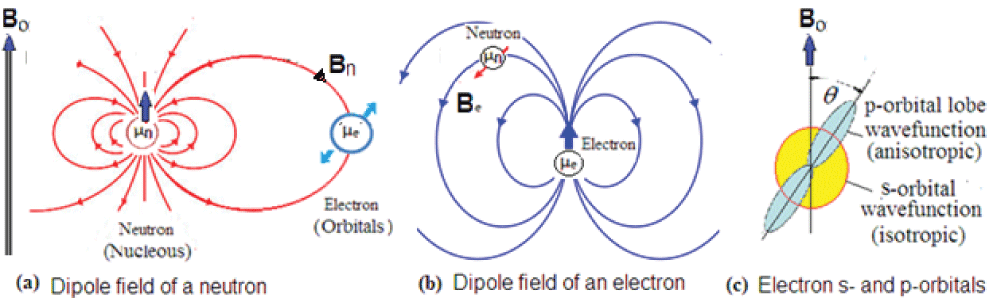
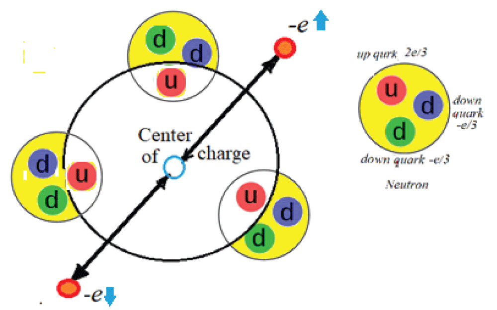
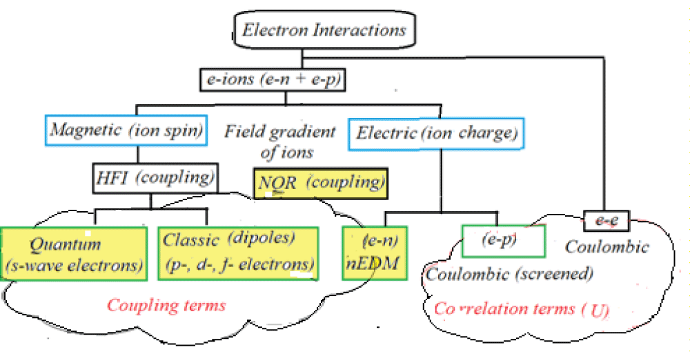
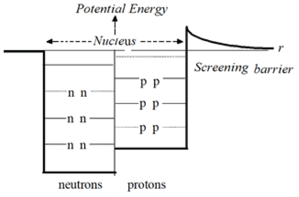
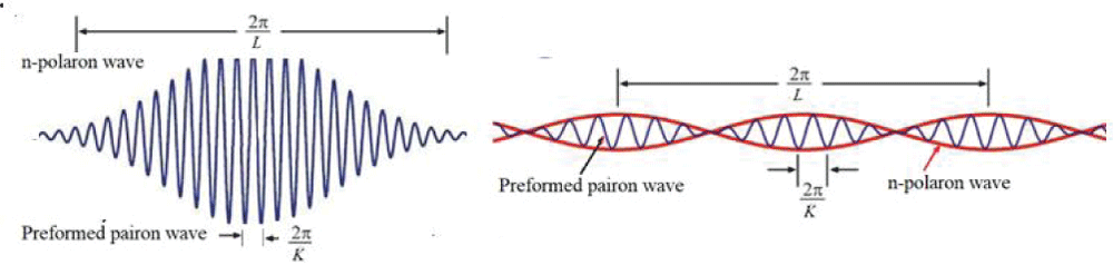
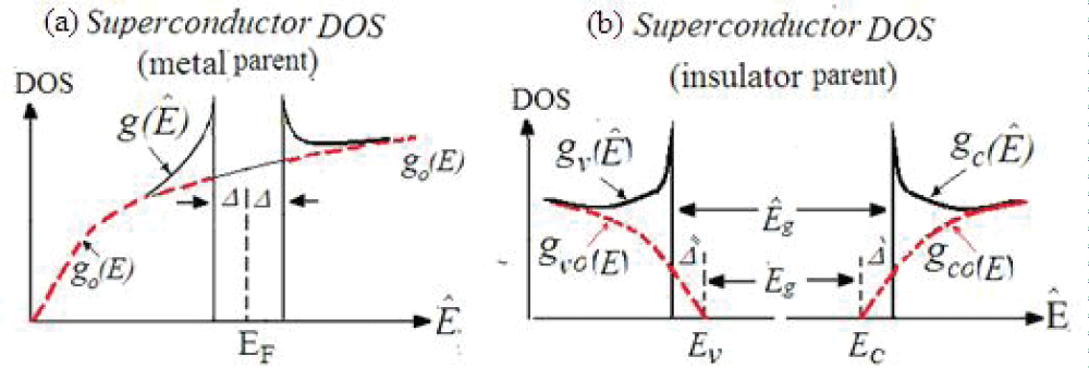
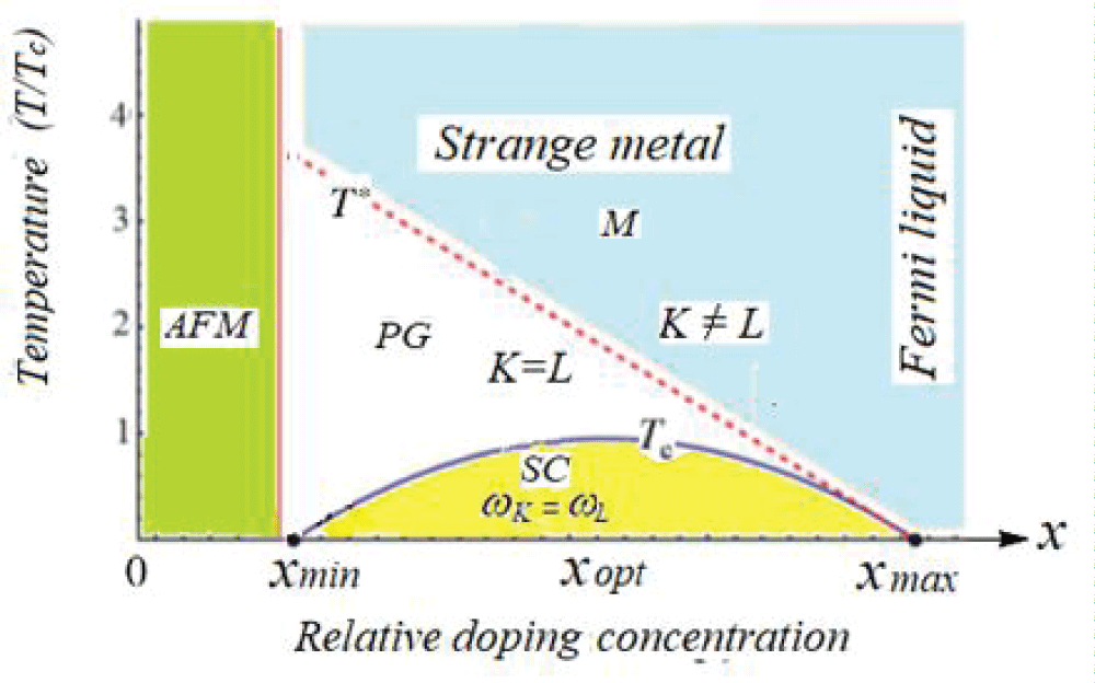
![(a) Experimental temperature dependence of magnetic hyperfine fields in a pnictide superconductor, and according to our primary calculations. The symbols refer to measurements by Saitovitcht & Litterst [69]. (b) Temperature dependence of a fluorine-doped Fe-pnictide sample (LaFe1−xMnxAsO0.89F0.11 with x=0.5%) as derived from Mössbauer spectra. This Figure was reproduced with permission from [1].](https://www.igminresearch.com/articles/figures/igmin359/igmin359.g009.png)
![Schematic of the vortices in cored regions of a type-II superconductor (left) and their Abrikosov triangular configurations in an HTS by magnetic force microscopy at two different temperatures below <em>T<sub>c</sub></em> (right). This Figure was reproduced with permission from [77].](https://www.igminresearch.com/articles/figures/igmin359/igmin359.g010.png)
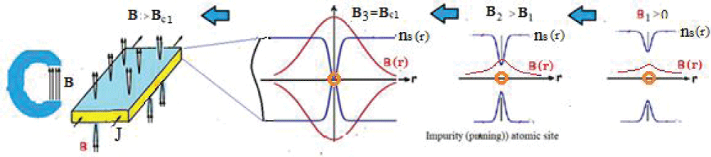
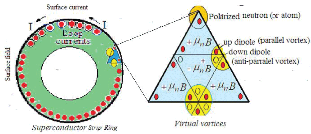
![Visualization of parallel and anti-parallel vortices in superconductors. Reproduced with permission from [78].](https://www.igminresearch.com/articles/figures/igmin359/igmin359.g013.png)

![Schematic diagram of the mechanisms of neutron-electron interactions of electromagnetic origin. QED stands for Quantum electrodynamics and QFD stands for Quantum Flavor dynamics. More details about QED and QFD can be found in [14].](https://www.igminresearch.es/articles/figures/igmin359/igmin359.g001.png)
![(a) Experimental temperature dependence of magnetic hyperfine fields in a pnictide superconductor, and according to our primary calculations. The symbols refer to measurements by Saitovitcht & Litterst [69]. (b) Temperature dependence of a fluorine-doped Fe-pnictide sample (LaFe1−xMnxAsO0.89F0.11 with x=0.5%) as derived from Mössbauer spectra. This Figure was reproduced with permission from [1].](https://www.igminresearch.es/articles/figures/igmin359/igmin359.g009.png)
![Schematic of the vortices in cored regions of a type-II superconductor (left) and their Abrikosov triangular configurations in an HTS by magnetic force microscopy at two different temperatures below Tc (right). This Figure was reproduced with permission from [77].](https://www.igminresearch.es/articles/figures/igmin359/igmin359.g010.png)
![Visualization of parallel and anti-parallel vortices in superconductors. Reproduced with permission from [78].](https://www.igminresearch.es/articles/figures/igmin359/igmin359.g013.png)