Comparing Forecasting Models for Predicting Infant Mortality: VECM vs. VAR and BVAR Specifications

Abstract

This study investigates infant mortality in Uganda, a persistent public health challenge in many developing countries where economic disparities limit access to healthcare. It compares the forecasting performance of three econometric models; Vector Error Correction Model (VECM), Vector Autoregressive (VAR), and Bayesian VAR (BVAR) using annual data on infant mortality rates (IMR), neonatal mortality rates (NMR), GDP, and GDP per capita (GDPP) from 1954 to 2016. Model accuracy was evaluated using Mean Squared Error (MSE), Root Mean Squared Error (RMSE), and Theil’s U-statistic.

The results show strong long-term relationships among IMR, NMR, GDP, and GDPP. VECM provides the most reliable long-term forecasts, with an adjusted R-squared of 97.7%. Impulse response analysis indicates that GDP increases IMR in the short run, while GDPP exerts a stronger long-term reducing effect. For NMR, GDP has a negative impact, whereas GDPP shows a gradual positive response over time. Granger causality tests reveal bidirectional causality between GDPP and IMR, and a unidirectional influence of IMR on GDP.

Uganda’s IMR is projected to fall to about 17 deaths per 1,000 live births by 2035, though NMR declines will slow. Policymakers should use VECM for long-term planning due to its superior accuracy and the strong cointegration among IMR, NMR, GDP, and GDPP, while VAR/BVAR can guide short-term monitoring. Because GDPP most strongly reduces mortality, welfare-enhancing strategies such as social protection and employment are crucial. GDP gains should fund maternal and neonatal health, and systems must be strengthened to withstand economic shocks.

Introduction

Infant mortality remains a critical global health challenge, particularly in developing regions such as Sub-Saharan Africa, where millions of children continue to die before their fifth birthday despite decades of progress. Infant mortality (IMR) and neonatal mortality (NMR) account for a large proportion of these deaths, which are often due to preventable or treatable causes such as neonatal encephalopathy, infections, complications from preterm birth, and malnutrition. In 2019 alone, over 5 million children under five died, with neonatal deaths declining more slowly than post-neonatal deaths [1-3]. In countries like Uganda, IMR and NMR remain high despite interventions aimed at improving healthcare access, such as mosquito nets, oral rehydration therapy, and maternal health programs. Key determinants of infant health include maternal education, per capita income, health expenditure, and environmental conditions [4]. The impact of macroeconomic factors on infant mortality is also evident, as studies show GDP fluctuations and economic growth influence maternal and child health outcomes, particularly in low-income countries where health system performance is critical [5].

In this context, examining how these factors interrelate with mortality rates becomes essential for designing effective policies aimed at achieving the SDG target of reducing under-five mortality to 25 per 1,000 live births by 2030 [6]. The causal effect of maternal and child mortality on GDP is generally stronger in HICs and UMICs due to the differences between poor and rich countries with respect to the human capital level or infrastructure. Human capital is the stock of competencies, knowledge, and social and personality attributes, including creativity, embodied in the ability to perform labor so as to produce economic value. The higher human capital level of richer countries compared to poorer countries implies that an equal reduction in maternal and child mortality will cause GDP to increase more in richer countries than in poorer countries [7].

Erdil, et al. [8] applied the Granger-causality approach to a panel data model with fixed coefficients in order to determine the relation between GDP and health expenditures per capita. They found significant bidirectional causality even for such a short time period, signaling that the evidence may be stronger for longer time periods. However, this causality is not homogenous, which is evident from the tests of the HC hypotheses. For one-way causality, the pattern of causality is different in low- and middle-income countries as compared to high-income countries. One-way causality generally runs from GDP to H in LIC and MIC, whereas the reverse holds for HIC.

The mortality‑forecasting literature suggests that univariate approaches such as ARIMA often overlook important interactions with other explanatory factors (e.g. socioeconomic or economic indicators), whereas multivariate models can capture these dependencies. For instance, Modeling mortality with a Bayesian vector autoregression [9] applies a multivariate Bayesian VAR (BVAR) to age‑specific mortality parameters and shows gains in forecast accuracy compared to simpler univariate methods. Evidence from a more recent study, Markov‑Switching Bayesian Vector Autoregression Model in Mortality Forecasting [10], demonstrates that adopting a regime‑switching multivariate framework (MSBVAR) further improves predictions and better accounts for structural changes in mortality patterns a scenario analogous to yours where infant/child mortality may respond dynamically to economic shifts (GDP, GDP per capita, etc.). Meanwhile, broader evidence from macroeconomic forecasting confirms that no single modelling approach uniformly dominates across settings: as noted in the review Forecasting in Economics and Finance, forecasting performance varies by variable, time‑horizon, and structural context, justifying a comparative modelling strategy rather than reliance on a single method.

Literature review

Forecasting models in health economics

Econometric models have increasingly been applied to forecast health outcomes such as Infant Mortality Rates (IMR) and Neonatal Mortality Rates (NMR). These models are useful in capturing complex interactions between socioeconomic and macroeconomic factors affecting health. Among the most commonly used techniques are Vector Error Correction Models (VECM), Vector Autoregressive (VAR) models, and Bayesian VAR (BVAR) models, each with unique strengths in modeling both short- and long-term effects and handling uncertainty in dynamic systems.

Recent studies demonstrate the application of various forecasting models in different contexts. In India, Mishra, Sahanaa, and Manikandan [11] used ARIMA models to forecast IMR from 1971 to 2016, predicting a decline to 15 deaths per 1,000 live births by 2025. Similarly, Khan, et al. [12] applied log-log regression and ARIMA models for Asian countries, showing strong correlations between IMR and GDP per capita. In Nigeria, Usman, et al. [13] found a decline in newborn mortality from 51.7% in 1990 to 33.9% in 2017 using ARIMA models, while Ogedi, et al. concluded that ARIMA outperformed Simple Exponential Smoothing (SES) and Brown’s Linear Trend (BLT) in forecasting NMR. These studies underscore the utility of time series models in projecting mortality trends, while also highlighting the potential for more advanced models to improve accuracy.

Vector Error Correction Models (VECM)

VECM is particularly effective for examining long-term relationships among non-stationary, cointegrated time series such as GDP, GDP per capita, and mortality rates. It allows researchers to analyze both short- and long-run dynamics, making it ideal for health economic applications. For example, Lin and Lee [14] applied VECM to healthcare spending and life expectancy, revealing strong long-term relationships between economic factors and health outcomes. Similarly, Sulaiman and Salleh [15] demonstrated that socioeconomic improvements, such as increased income, contributed to sustained reductions in infant mortality. Studies in Greece and other settings confirm that VECM effectively captures long-term dependencies and enhances forecasting accuracy compared to univariate models like ARIMA [16-18].

Vector Autoregressive (VAR) Models

VAR models analyze interdependencies among multiple variables without assuming cointegration or a specific causal direction. This flexibility makes them suitable for examining how macroeconomic variables, including GDP and GDP per capita, influence IMR and NMR over time. Liao, et al. [19] used VAR to show significant links between health expenditures, economic growth, and life expectancy in China. In sub-Saharan Africa, Imo, et al. [20] found that short-run variations in IMR were influenced by healthcare investments, whereas long-term improvements required broader socioeconomic development. VAR models have also highlighted the differential impact of GDP per capita and health spending on under-five mortality, demonstrating their value in forecasting short-term dynamics and feedback effects [21-23].

Bayesian VAR (BVAR) Models

BVAR extends traditional VAR by incorporating Bayesian methods to improve estimation under uncertainty and limited data. By including prior knowledge, BVAR models provide more robust forecasts, particularly for long-term health trends [24]. Applications in low-income countries show that BVAR delivers accurate predictions despite data limitations, allowing policymakers to incorporate factors such as maternal education, sanitation, and healthcare spending [25,26]. Studies in Australia further confirm that BVAR outperforms traditional VAR models by accounting for parameter uncertainty, particularly when projecting long-term mortality trends [9,27].

Comparison of VECM, VAR, and BVAR Models

While VECM, VAR, and BVAR are widely applied in health forecasting, few studies comprehensively compare their performance in predicting IMR and NMR. Fernández, et al. [28] found that BVAR models generally provide more accurate forecasts under uncertainty, whereas Dube, et al. concluded that VECM captures long-term relationships more effectively, with VAR better suited for short-term forecasting. Comparing these models is crucial for identifying the most reliable approach to inform policy and resource allocation, particularly as countries aim to meet SDG targets for child health. Accurate forecasting supports evidence-based decision-making for healthcare interventions, long-term planning, and socioeconomic strategies to reduce infant and neonatal mortality.

Methods

Data sources

The study utilized country-specific annual infant and neonatal mortality rates data compiled and provided by http://www.childmortality.org. UN IGME web site data used in the United Nations Children’s Fund (UNICEF) Report on levels and trends in Child Mortality. Data on Ugandan GDP and GDP per capita was obtained from the World Bank web site. The researchers used GDP at 2000 US prices (the World Bank’s World Development Indicators 2016; http://devdata.worldbank.org/wdi2016.htm).

Procedures

The projection of infant and neonatal mortality based on the vector error correction model from 2030 was done using time series data from 1954 to 2016, collected from UNICEF, the Bank of Uganda. Variables considered here include: infant mortality rate, neonatal mortality rate, country’s GDP per capita, and GDP.

Forecasting the infant and neonatal mortality

Three stages of analysis were adopted to facilitate the achievement of the goal. In the first stage, the study examined the trends and patterns of infant and neonatal mortality rates, government health expenditure, GDP, GDP per capita, sanitation coverage, and maternal literacy levels. The study was further focused by conducting an optimal lag length determination and a co-integration test. The second stage involved time series analysis (VAR, BVAR, and VECM) in order to determine the relationships and effects of the aforementioned variables on health outcomes. Lastly, the study devoted stage three to performing an out-of-sample projection of infant and neonatal mortality rates in 2030.

Time series analysis was used to identify the magnitude and direction of the relationship between health outcomes and GDP, GDP per capita, government health expenditure, sanitation coverage, and maternal literacy.

Statistical analysis

Trend and patterns of infant and neonatal mortality rates, Ugandan GDP, GDP per capita were explored through graphs.

Stationarity assessment of the variables

All the series (IMR, NMR, GDP, and GDPP) were tested for stationarity before they were fixed into the model. According to Granger and Newbold [29], if there is a unit root, then that particular series is considered non-stationary.

A stochastic time series Yt is said to be stationary, if and only if, it satisfies the following assumptions:

1. $E\left(Y_t\right)=\mu$

2. $Var\left(Y_t\right)={\delta }^2$

3. $Cov\left(Y_t{Y}_{t-1}\right)={\delta }^k$

Conditions (1) and (2) imply that has a constant mean and variance over time, while condition (3) means that the covariance between series depends only on how far apart they are and not on the time of occurrence [30]; Box and Jenkins [31]. If one or more of the above conditions are not satisfied, the series is non-stationary, and proceeding with regression analysis would result in spurious results, which can produce high t-statistics but have no coherent economic meaning or an insignificant result.

Dicky fuller unit root test for stationarity in the series

The Augmented Dicky-Fuller (ADF) standard test for unit root in the series was used in testing for the presence of unit root in both transformed and non-transformed series. The time series data in this study can take any of the following stationarity models:

$\Delta Y_t=\gamma Y_{t-1}+{\epsilon }_t$ (Radom walk) (1)

$\Delta Y_t={\sigma }_0+\gamma Y_{t-1}+{\epsilon }_t$ (Random walk with a drift) (1.2)

$\Delta Y_t={\sigma }_0+{\sigma }_2+\gamma Y_{t-1}+{\epsilon }_t$ (Mixed process) (1.3)

The error terms εt are assumed to be independent and identically distributed. Dickey and Fuller [32] proposed the ADF test in order to handle the autoregressive process in the variables [33]. Where the ADF indicated the occurrence of a unit root, then the series is non-stationary. In case of non-stationary, then the researcher proceeded to taking the logarithms, differencing until he arrives at a stationary series.

Many scholars used differencing to detrend the data and control autocorrelation by subtracting each datum in a series from its predecessor until stationarity was attained [34]. Once stationarity is attained after differencing d times, the series is said to be integrated in order d [35]. In such cases, the researcher then proceeded with optimum lag length determination and co-integration analysis.

Model specification and identification

The first step in building a VAR (p) model involved model identification. This helps in identifying the appropriate model's order. The most common methods used for lag order determination include Akaike Information Criterion (AIC) [31], Schwarz-Bayesian (BIC), and Hannan-Quinn (HQC). The main idea of AIC is to select the model that minimizes the negative likelihood penalized by the number of parameters.

The AIC and SBC equations are given below:

$AIC=Tlog\left|{{\displaystyle \sum }}^{\text{}}\right|+2N$ (1.4)

$SBC=Tlog\left|{{\displaystyle \sum }}^{\text{}}\right|+Nlog\left(T\right)$ (1.5)

Where;

|Σ| = The determinants of the variance/covariance matrix pf the residuals;

N = Total number of parameters estimated in all equation; and

T = The number of usable observations.

Both AIC and SBC differ in their exact definition of a good model. In this case, the study chooses the model that has the lowest AIC and SBC values.

The time series Yt, where $Y_t=(Y_{1t},Y_{2t},\dots \dots \dots \dots \dots \mathrm{..}, Y_{nt})$ denote an (n × 1) vector variables, follows a VAR(p) model if it satisfies

$Y_t={{\displaystyle \prod }}^{\text{}}+{\Phi }_1{Y}_{t-1}+\dots \dots \dots \dots \dots +{\Phi }_{t-p}{Y}_{t-p}+e_t , t=1,2,3,\dots .t$ (1.6)

Matrix expression of equation 1.6 is as follows,

$\begin{array}{l}\left[\begin{array}{c}{y}_{1t}\\ y_{2t}\\ :\\ y_{nt}\end{array}\right]=\left[\begin{array}{c}{\Pi }_1\\ {\Pi }_2\\ :\\ {\Pi }_n\end{array}\right]+\left[\begin{array}{cccc}{\Phi }_{11}^1& {\Phi }_{12}^1& \mathrm{...}& {\Phi }_{1n}^1\\ {\Phi }_{21}^1& {\Phi }_{21}^1& \mathrm{...}& {\Phi }_{2n}^1\\ :& :& \mathrm{...}& :\\ {\Phi }_{n1}^1& {\Phi }_{n2}^1& \mathrm{...}& {\Phi }_{nn}^1\end{array}\right]\left[\begin{array}{c}{y}_{1t-1}\\ y_{2t-1}\\ :\\ y_{nt-1}\end{array}\right]+\left[\begin{array}{cccc}{\Phi }_{11}^2& {\Phi }_{12}^2& \mathrm{...}& {\Phi }_{1n}^2\\ {\Phi }_{21}^2& {\Phi }_{21}^2& \mathrm{...}& {\Phi }_{2n}^2\\ :& :& \mathrm{...}& :\\ {\Phi }_{n1}^2& {\Phi }_{n2}^2& \mathrm{...}& {\Phi }_{nn}^2\end{array}\right]\left[\begin{array}{c}{y}_{1t-1}\\ y_{2t-1}\\ :\\ y_{nt-1}\end{array}\right]+\mathrm{....}\\ \left[\begin{array}{cccc}{\Phi }_{11}^p& {\Phi }_{12}^p& \mathrm{...}& {\Phi }_{1n}^p\\ {\Phi }_{21}^p& {\Phi }_{21}^p& \mathrm{...}& {\Phi }_{2n}^p\\ :& :& \mathrm{...}& :\\ {\Phi }_{n1}^p& {\Phi }_{n2}^p& \mathrm{...}& {\Phi }_{nn}^p\end{array}\right]\left[\begin{array}{c}{y}_{1t-1}\\ y_{2t-1}\\ :\\ y_{nt-1}\end{array}\right]+\left[\begin{array}{c}{e}_{1t}\\ e_{2t}\\ :\\ e_{nt}\end{array}\right]\end{array}$

Where Π is a k-dimensional vector, Φ₁, Φ₂,…….,Φ_p are k*k parameter matrices and et is a sequence of independently and identically distributed error vector.

Assumptions of the errors: -

The error term et is a multivariate normal k*1 vector of error satisfying the following assumptions;

1. E (e_t) = 0; every error term has a mean zero;

2. E(e_t e'_t) = s the contemporaneous covariance matrix of error terms is ω (an*n positive semi-definite matrix);

3. For any non-zero k. There is no correlation across time; in particular, no serial correlation in individual error terms and Φ_j are k*k matrices.

Lag length determination and model selection

Lag selection for IMR and NMR was conducted using AIC, BIC, and HQC, guided by inspection of ACF/PACF plots. The two-mortality series exhibited different autocorrelation structures, which justified the use of different maximum lag lengths. Stationarity was assessed using ADF tests, and non-stationary I (1) variables were retained for cointegration testing using the Johansen trace and max-eigenvalue procedures. Where cointegration existed, variables were modelled using VECM; otherwise, differenced stationary series were used in VAR and BVAR. Non-stationary variables were not excluded because cointegration analysis requires I (1) variables to estimate long-run relationships. Both the Chao and Phillips joint procedure and the Johansen-Juselius sequential approach were applied to determine the cointegration rank, ensuring robustness of the long-run specification.

Lag length determination

Four basic variants of the model were estimated:

(i) the VEC model using both the Chao and Phillips, 1999 joint procedure, VEC(J), and the more standard sequential procedure based on using the BIC to select the lag length and Johansen and Juselius’s, 1990 maximum root test to select the number of common trends using a sequence of 5% tests, VEC(S).

(ii) A VAR using BIC to select the lag length.

(iii) A DVAR using BIC to select the lag length.

(iv) Two BVARs, each using AIC to select the lag length, but with either the standard Minnesota priors (with hyper parameters of 0.2 for the diagonal and 0.2 for the off-diagonal terms), BVAR (M), or with looser priors on the off-diagonal (off-diagonal hyper parameter = 0.8), BVAR (L).

Vector autoregressive processes

According to Sims, 1980 and Litterman [34], Vector Autoregressive (VAR) models have been proven to forecast better than any simultaneous equation models. Vector Autoregressive (VAR) models provide information about a variable’s forecasting ability for another variable. It is an econometric model used to capture the evolution and the interdependence between multiple time series. In order to build a VAR model [31], certain steps can be followed. This includes model identification, estimation of constants, a diagnostic check, and finally forecasting. Conditional heteroscedasticity and outliers in the residual series are also checked. The existence of co-integration was used to check for the presence of any common trends, and finally, an Error Correction Model (ECM) was developed due to presence of co integration to improve the long-term forecast.

Estimation of the VAR model

After obtaining the order of the model, p, of the vector series, the researcher derived the estimators of the constants as in the steps below.

Consider the consecutive VAR models:

$Y_t={{\displaystyle \prod }}^{\text{}}+{\Phi }_1{Y}_{t-1}+e_t ,$

$Y_t={{\displaystyle \prod }}^{\text{}}+{\Phi }_1{Y}_{t-1}+2Y_{t-2}+e_t ,$

…=…

$Y_t={{\displaystyle \prod }}^{\text{}}+{\Phi }_1{Y}_{t-1}+2Y_{t-2}\dots \dots \dots +{\Phi }_i{Y}_{t-i}+e_t ,$ (1.7)

The most common methods of estimating parameters are the maximum likelihood estimator (MLE) and the ordinary least squares estimator. Here, the study applied the ordinary least squares (OLS) method to estimate the parameters of these models and applied equation by equation.

For equation (1.7), let ${\Phi }_i^{(j)}$ be the OLS estimate of Φ₁ and ${\widehat{\prod }}_i^{(j)}$ be the OLS estimate of Π. Where (i) is used to denote the estimate of a VAR (i) model. The estimates of the coefficients of the VAR model. ${\Phi }_1{\widehat{Y}}_{t-1}+\dots \dots \dots \dots +{\Phi }_{\text{p}}{\widehat{Y}}_{t-p}+e_t ,$ When estimated using the unrestricted VAR (p) model are considered to be fixed quantities. These estimates of coefficients do not accurately reflect the underlying relationship because some of the estimated coefficients of the VAR model are non-zero purely by chance when estimated by OLS so restrictions may be imposed to reduce the number of parameters being estimated, Mercy, et al. 2015.

Diagnostic check for VAR model

Suppose the orders and constants have been chosen for a VAR model underlying the data, then residuals are checked to see whether they are normally, identically, and independently distributed. After the model had been fitted, heteroscedasticity was tested through multivariate arch tests; autocorrelation through Durbin Watson; normality through Jarque-Bera tests; the unit root test through the Dickey Fuller and Augment Dickey Fuller tests; and the statistical significance of the parameters was tested through t statistics. For details, look at Mercy, et al. 2015.

Data description

Standard practice in VAR analysis is to report results from Granger causality tests, impulse responses, and forecast error variance decompositions. These statistics are computed automatically (or nearly so) by many econometrics’ packages. Because of the complicated dynamics in the VAR, these statistics are more informative than the estimated VAR regression coefficients or statistics, which typically go unreported. Granger-causality statistics examine whether lagged values of one variable help to predict another variable.

Bi-variate Granger causality was used to determine which national variables help predict health outcomes. If a variable Granger causes a health outcome, it is included in the VAR and BVAR forecasting models. These tests were conducted for each health outcome at lag length 1,2,3,4 and 5 years using both a deterministic time trend and first differences.

Forecasting models

Bayesian Vector Autoregressive (BVAR) was used in this study to assess whether prior information on spatial and economic base-sectoral linkages improves forecast accuracy for health outcomes in Uganda. The study then forecasted the mortality levels using VAR and BVAR

models to compare their forecasting accuracy.

Assessment of forecast performance or VAR and BVAR

Alkema and New [35] concluded that, point estimates on child mortality based on limited information may substantially under- or overestimate the truth. Uncertainty assessments can and should be used to complement point estimates to avoid unwarranted conclusions about levels or trends in child mortality and to reduce confusion about differences in estimates within and between countries. In this study, both bootstrapping and cross-validation were used to assess the predictive power of the models, and the best model was used to project the infant and neonatal mortality by 2030 or 2035.

Infant and neonatal mortality forecasts

Time series analysis uses the factor of time to replace other kinds of influencing factors. Li Y, et al., used the autoregressive integrated moving average (ARIMA) model, one of the classic methods of time series analysis based on past values of a series and previous errors, to forecast under-five mortality in India. Despite all the advantages of this approach, it does not consider the influence of other macro variables in the economy like the Vector Auto Regressive model. The study then considered the infant and neonatal mortality rates from 1954 to 2014 as a training sample to fit the VAR model, and 2015–2017 was considered for the within and without samples for internal and external validation, respectively.

To compare the performance of the VECM, VAR and BVAR models, the researcher computed the mean square error, root mean square error, and Theil’s U statistics for the quality of the time series forecast methods.

For a VAR(p) model, the 1-step ahead forecast at the time origin h is given by;

$Y_h\left(1\right)={{\displaystyle \prod }}^{\text{}}+{\displaystyle \sum }_{i=1}^p{\Phi }_i{Y}_{h+1-i}$ (1.8)

The associated forecast error is ah = eh +1

The covariance matrix of the forecast error is Σ. If Y_t is weakly stationary, then the 1-step ahead forecast Y_t(1) converges to its mean vector, µ, as the forecast horizon increases, Mercy, et al. 2014.

(i) Mean Squared Error (MSE): Any of the two models was considered best if it has the minimum forecast error arising from comparing the actual value and forecast value. $a_h=e_h+1MSE({\widehat{Y}}_t)=E{({\widehat{Y}}_t-Y_t)}^2$

(ii) Root Mean Squared Error (RMSE): Is the square root of the average of all squared errors, according to Wang and Lim 2005. It ignores any over and under- estimation.

(iii) Theil’s U Statistic: Theil's U-statistics see Theil, 1958 is used as a measure of forecasting error that is minimized. It is a relative measurement based on comparison of the predicted change with the observed change. The value of U lies between 0 and 1. If U equals to 0, there is a perfect fit, whereas U equals to 1 implies that forcasting of data is very poor.

Assessment of the forecasting accuracy of BVAR, VECM and VAR model

However, the forecast of infant mortality from 2030 forward is very important in knowing what infant and neonatal mortality would look like if nothing is done to address the risks of infant and neonatal mortality. This paper provides exploratory results on the forecasting powers of three econometric models such as BVAR, VECM, and VAR in estimating the future IMR and NMR in Uganda based on historical data.

Forecast Error Variance Decomposition (FEVD)

To understand the relative importance of different shocks in the system, we applied Forecast Error Variance Decomposition (FEVD) to the VAR/VECM models. FEVD quantifies the proportion of the forecast error variance of each dependent variable (IMR, NMR) that can be attributed to innovations in itself versus innovations in other variables (GDP, GDPP) over different time horizons. This allows us to identify which variables drive fluctuations in infant and neonatal mortality in the short and long run, and how the influence of each variable evolves over time. The method complements impulse response analysis by providing a quantitative measure of each shock’s contribution to overall variability [36-38].

Results

Lag length for modelling IMR

The maximum lag length of five (5) was chosen based on the lowest value of AIC, FPE, LR, and HQIC to model IMR (Table 1).

Similarly, a maximum lag length of four (4) was determined based on the same approach to model NMR in Uganda (Table 2).

Determination of the direction and magnitude of the relationships between health outcomes and macroeconomic variables

Given that the study focused on two health outcomes (IMR and NMR), we selected the appropriate model for assessing the relationship between health outcomes and independent variables.

Choice of model

Chepngetich and John, 2015 reported that VAR models are used to describe and forecast multivariate time series for stationary time series and recommended that for non-stationary time series, a vector error correction term is added to form a vector error correction model (VECM). It was therefore necessary to test for the existence of a stationary linear combination of the non-stationary terms (co-integration). I transformed the selected series into a vector error correction model (VECM) by taking the first difference, which in turn facilitated long-term forecasting. Those series that were not stationary at the first difference were dropped from the forecasting model.

Vector auto regressive model to assess the relationship between IMR and GDP, GDPP

Understanding how the variables relate to changes in the outcome variables is important in planning and policy formulation. As a result, I investigated the relationship between LIMR, LNMR, LGDP, and LGDPP. 

Impulse response

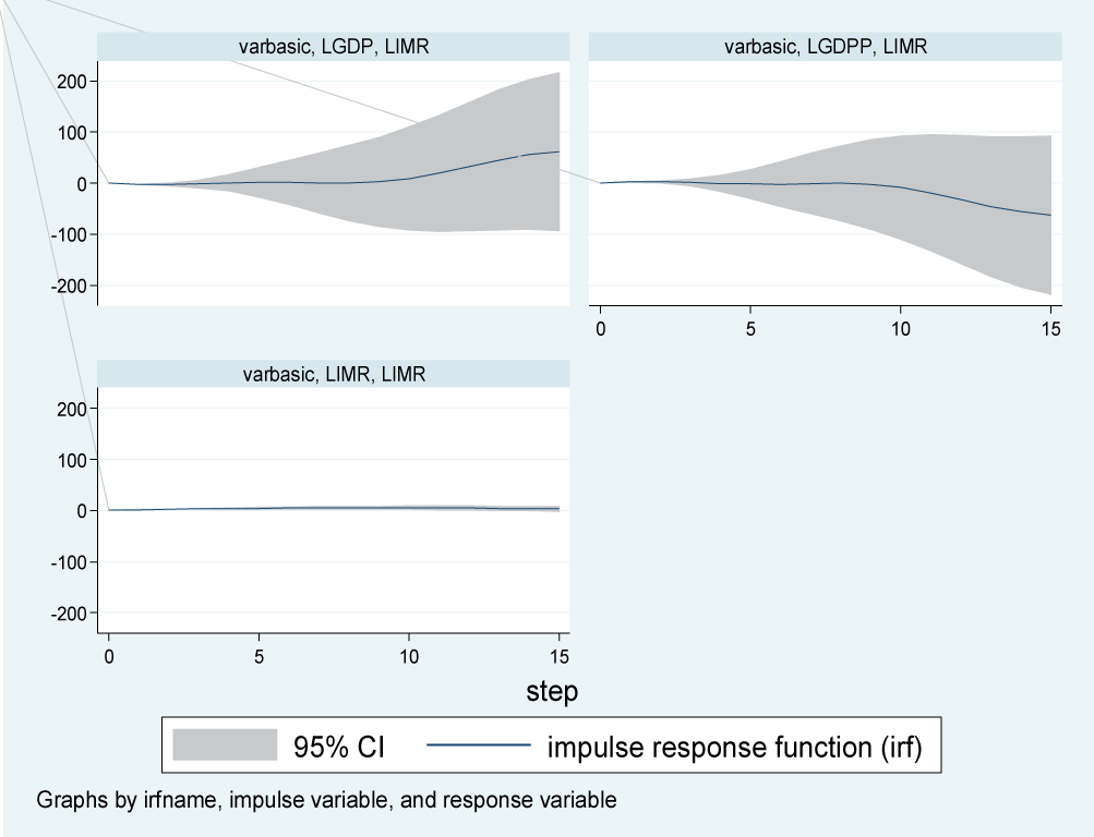
The first step taken in building a VAR (p) model was the identification of the appropriate model (lag length) using the Akaike Information Criterion (AIC). The main idea of AIC is to select the model that minimizes the negative likelihood penalized by the number of parameters. The VAR model was then fitted to investigate how changes in the independent variables (LGDP and LGDPP) could affect the health outcomes (LIMR and LNMR) as presented in Figure 1. 

The response of LIMR to a one standard deviation (SD) shock (innovation) in LGDP remained steady at about zero in the first five years and increased slightly in the subsequent five years; however, beyond 10 years, LIMR rose above average quickly as compared to the previous period and it remains in the positive region. That is, shocks to LGDP will have a positive impact on LIMR in both the short and long run. Furthermore, the effect of a one SD shock in the LGDPP was not noticeable in the short run and declined in the negative region slowly in the period between five and ten years, but it decreased rapidly beyond 10 years. This implied that the shock to LDGPP will have a negative impact on LIMR in the long run; that is, an increase in a country’s GDPP leads to an increase in health infrastructure development in the long run, which in turn leads to a drop in infant mortality (Figure 1).

Impulse response of NMR to a one SD shock on LGDP and LGDPP

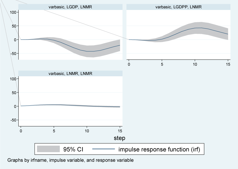
The response of LNMR to a one SD shock (innovation) on LGDP was about zero in the first three years, and it decreased rapidly between three and ten years; it remained steady between 10 and twelve years. Beyond twelve years, LNMR registered a quick rise but remained in the negative region. In other words, a one SD shock in LGDP hurts LNMR in both the short and long run (Figure 2).

Similarly, while the impact of a one-SD shock in LGDPP on LNMR was not noticeable in the period zero to five years, the response rapidly increased between the five- and ten-year periods, where it hit a steady value for about two years. The response of LNMR to stimulation in LGDPP started declining but remained in the positive region beyond 12 years. This meant that a shock to LGDPP would benefit LNMR in both the short and long run (Figure 2). 

Engle granger causality GDP and GDPP on Health outcome (IMR and NMR)

Based on variables such as IMR, GDP, and GDPP, it was noted that GDPP significantly influences IMR in the short run. In addition, Uganda's GDP and GDP all together cause changes in IMR in the short run. In a similar twist, it was discovered that IMR causes GDP, yet GDPP was found not to be significant in causing GDP. It's worth noting that both IMR and GDPP influence a country's GDP. It was also observed that IMR significantly causes GDPP and that there were no significant causal effects between GDP and GDPP (Table 3).

The findings revealed a significant two-way causality between IMR and GDPP and a one-way causal effect from IMR to GDP. Interestingly, it was clear that GDP only causes IMR through GDP. There was no causality between GDP and GDP in the short term. In view of the above, four variables that caused an increased infant or neonatal mortality rate were included in the VAR, VECM, and BVAR models.

There was a strong relationship between health outcomes (such as IMR and NMR) and GDP, just like GDPP, which could be due to the level of human capital dependency and the higher marginal effect of health spending on LIC and LMIC. This was in agreement with the research conducted by Amiria and Gerdtham, 2013, who found that there was a stronger relationship because the effects of GDP on health are stronger in LIC and LMIC compared to HIC and UMIC, while, in contrast, the effects of health on GDP are stronger in HIC and UMIC compared to LIC and LMIC. The tests were run with a lag length of four for neonatal mortality and five for infant mortality as predetermined in lag length selection procedures (Table 3).

The Granger causality test was employed to determine whether lagged values of GDP (LGDP) and GDP per capita (GDPP) could predict infant mortality rate (LIMR) and neonatal mortality rate (LNMR). The findings indicate a strong causal relationship, as the lagged values of both LGDP and GDPP significantly influence LIMR, with p-values less than 0.001. This suggests that changes in GDP and GDP can effectively predict future infant mortality rates in the short term. Furthermore, a direct causal effect of LGDP and GDPP on LNMR was also observed, confirming that these variables are useful for forecasting neonatal mortality rates. However, the lagged values of LNMR did not independently affect LGDP, but they did show a significant effect when combined with LGDPP (p = 0.017). Similarly, LIMR did not exhibit a direct causal effect on GDPP alone, but this relationship became significant when considering the interaction with LGDP. Overall, while LNMR has a significant influence on both LGDP and GDPP, the direct causal relationships among these variables highlight the complex interdependencies in predicting mortality rates in the context of economic factors (Table 3).

Johansen cointegration test

IMR, NMR, GDP, and GDPP were among the variables taken into account in this study. They were non-stationary at the level but became stationary after the first difference. Based on these results, I used the Johansen test of co-integration at 5% to check for co-integration. This assisted in determining whether the variables move together over time or not, which in turn assisted in choosing between fitting the VAR model and the VECM. Results revealed that there was an order 1 co-integration between LIMR, LGDP, and LGDPP, as well as an order 2 co-integration between LNMR, LGDP, and LGDPP. This meant that these three variables move together in the long run, hence the need to fit the Vector Error Correction Model (VECM) for both NMR and IMR.

Assessment of the forecasting performance of VECM and BVAR

To keep things simple, the analysis results showed that there was co-integration of order one for infant mortality data (IMR) and order two for neonatal mortality data (NMR). The study considered the first order of co-integration in the subsequent analysis. With the presence of co-integration in the data set, VECM was found to be more appropriate for making long-term projections than the VAR model, whose supremacies were observed only in the short run. However, there was a need to compare the projection accuracy between VECM and BVAR (Table 4).

To accomplish this, the dataset was divided into two parts (the training data was sampled from 1954 to 2010, and the validation data was sampled from 2011 to 2018). The accuracy levels for within-sample forecasts were assessed using Root Mean Squared Error (RMSE), Mean Absolute Error (MAE), Mean Absolute Percent Error (MAPE), and the Theil Inequality Coefficient. In all cases, the model with the minimum possible errors was taken to be the best (Table 4).

The results in Table 4 revealed that, in the long run, the model that can best predict infant mortality rate in Uganda is VECM since it has smaller values of the projection errors as compared to BVAR.

Table 5 indicates that the Vector Error Correction Model (VECM) demonstrated superior accuracy in projecting neonatal mortality rates, as evidenced by its lower forecast error values compared to the Bayesian Vector Autoregression (BVAR) model. Consequently, VECM was selected for forecasting infant and neonatal mortality rates from 2021 to 2035. The study further explored the relationships among Infant Mortality Rate (IMR), Neonatal Mortality Rate (NMR), Gross Domestic Product (GDP), and GDP per capita (GDPP) to assess the impact of changes in GDP and GDPP on IMR and NMR. To quantify this effect, forecast error variance decomposition was employed, measuring the extent to which variations in GDP and GDPP account for changes in IMR and NMR over both short and long-time horizons.

Infant mortality rate in VECM

Based on the long-run equation, it was clear that LGDP hurts IMR, whereas GDPP has a positive effect on infant mortality, and the coefficients were significant at the 5% level. In a nutshell, LGDP and LGDPP have a symmetric effect on LIMR in the long run, on average, ceteris paribus. Overall, the VECM fitted the data very well, with an adjusted R-squared of 97.7%. Further still, the F-statistics were significant at the 1% level (Table 6).

Diagnostic check

Results of the post-estimation tests indicated that the fitted model had no serial correlation at the 5% level of significance. However, the errors were not normally distributed based on the Jarque-Bera test, and no heteroscedasticity was seen based on the Breusch-Pagan-Godfrey test at the 5% level of significance. In addition, the VECM specification imposes 2-unit moduli, which implies a high level of stability at the significance level of 5% (Table 6)

Short-run causality

The results of the vector error correction model with IMR as the dependent variable showed no significant short-run causality from LGDP and LGDPP to IMR at a 5% level of significance. It was important to keep in mind that there was a short-run causal relationship between the IMR's lag values and its present values. IMR's values from the previous two years had a positive impact on its current value, which means that in the near future, IMR will grow by 68.5% and 60.4% on itself as a result of its first and second prior values, respectively. On the other hand, due to the impact of its values from three years ago at a 5% level of importance, IMR will show a decline of 51.9% in the short term (Table 7).

Long run causality for IMR

The adjustment term (-0.0041) suggested that previous year’s error (or deviation from long-run equilibrium) is corrected for within the current year at a convergence speed of 0.041% annually.

In the short run (6 years), more than 80% of the forecast error variance is explained by IMR itself, and very little influence is seen from GDP and GDPP. In the long run (10 to 15 years), the influence of the LGDP increases while that of the GDPP remains stagnant. This meant that GDP exhibited a strong influence on IMR in the long run, yet IMR had a weak endogenous influence on itself (Table 8).

Neonatal mortality rate in VECM

In the long run, LGDP has a negative impact on LNMR, while LGDPP has a positive impact on LNMR, and the coefficients are significant at the 1% level. In conclusion, I found out that LGDP and LGDPP have a symmetric impact on NMR in the long run-on average, ceteris paribus. The VECM fit the data very well overall, with an adjusted R squared of 97.7%; additionally, the F-statistics were significant at the 1% level. 

Diagnostic check under NMR

The model's post-estimation results revealed no serial correlation; error terms were normally distributed, with no heteroscedasticity based on the Breusch-Pagan-Godfrey test at 5%; and the VECM specification imposed 2-unit moduli, implying a high level of stability (Table 9). 

Short-run causality

The VECM results revealed no short-run causality running from the lagged values of NMR; in particular, the current values of NMR tend to increase with neonatal mortality by 99%. Furthermore, there were no short-run causalities from lagged GDP and GDPP values to NMR because their coefficients were not significant at the 5% level, implying that there is no short-run causality from LGDP and LGDPP to LNM (Table 10).

Long-run causality

The VECM results showed an adjustment term of -0.014, suggesting that the previous year’s errors are corrected within the current year at a convergence speed of 1.4% annually, towards the long-run equilibrium. Furthermore, it indicated long-run causality running from LGDP and LGDPP to LNMR.

In the short run (1–6 years), the majority of the neonatal mortality forecast error variances (over 89%) were explained by themselves, and only a very small percentage was explained by GDP and GDPP. This influence reduced with time to the extent that, between 10 and 15 years, the influence of GDPP on NMR became stronger, and that of GDP remained weak all through the period (Table 11).

Forecast of infant and neonatal mortality in Uganda

After assessing the forecasting powers of the models, predictions for infant and neonatal mortality in the long run up to 2035 based on the Vector Error Correction Model (VECM) were estimated since it proved to be more reliable in making long-term forecasts (Table 12).

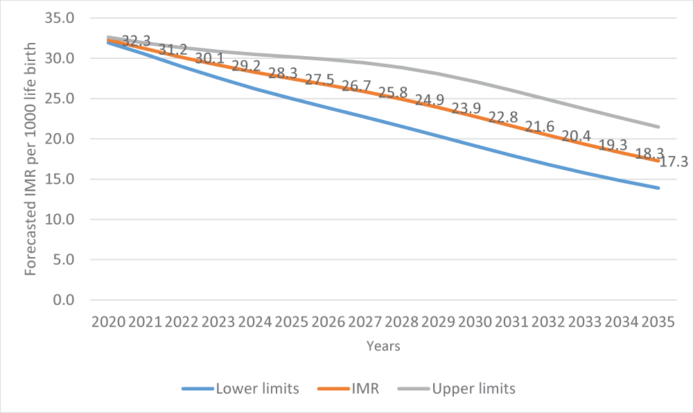
Globally, there has been a steady decline in NMR figures over the years, particularly in Uganda; however, this appears to have stalled in recent years, and this trend of slow decline is expected to continue during the lifespan of the Sustainable Development Goals if nothing is done. As presented in Figure 3, we applied the suitable prediction model (VECM) after a deeper investigation of its capability to conduct both the short- and long-term forecasts. It was observed that by 2035, Uganda will have about 17 deaths per 1,000 live births.

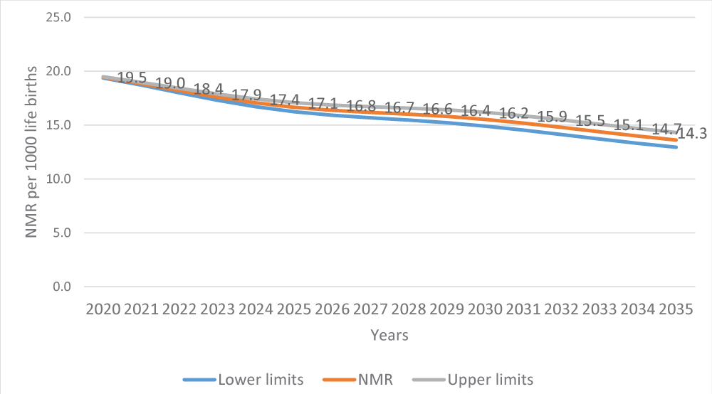
Results presented in Figure 4 show that the decline of NMR will continue to slow over the next 15 years. The projections presented here indicate where the health practitioner should focus. If the goal of eradicating infant mortality is to be realized, more emphasis should be placed on newborn life throughout the country. 

Discussion

The analysis of IMR and NMR in relation to GDP and GDP per capita (GDPP) revealed a significant negative correlation overall: as national GDP and GDPP increase, resources available for investment in the health sector expand, improving access to quality healthcare services and enhancing infant survival. Impulse response functions indicate that in the short run, the response of log-transformed IMR (LIMR) to a one standard deviation shock in LGDP is minimal, reflecting limited immediate impact. However, beyond ten years, LIMR rises and remains in the positive region, suggesting that shocks to LGDP exert a sustained long-term influence on infant mortality.

VECM long-run coefficients (p <  0.05) confirm a negative effect of LGDP on IMR, consistent with the expected economic-health link. Conversely, GDPP exhibits a positive long-term association with infant mortality, which may appear counterintuitive. This outcome can be attributed to structural and contextual factors: rising GDP does not guarantee equitable resource distribution. If economic growth primarily benefits wealthier households, marginalized populations may experience minimal improvements in health, nutrition, or sanitation. Rapid economic growth may also outpace investments in health infrastructure and maternal care, while urban overcrowding and environmental hazards persist, thereby offsetting potential mortality reductions. These findings underscore the importance of equitable growth and targeted health investments to translate economic gains into tangible health benefits.

The observed associations align with findings from Khan, et al. 2019, who forecasted IMR for Asian countries using log-log regression and ARIMA models, reporting significant correlations between GDP and IMR. Similarly, Ensor, et al. [5] highlighted those economic recessions negatively affect maternal and infant health, particularly in the early stages of national development. The relationship between GDP, GDPP, and infant mortality is also influenced by human capital; in low- and middle-income countries (LICs and LMICs), the marginal effect of health spending on mortality is higher, whereas in high- and upper-middle-income countries (HICs and UMICs), reductions in mortality have a stronger effect on GDP.

Comparative analyses of the SAARC countries further support these findings. Panel data analyses from 1990 to 2016 revealed that GDP per capita, health spending, and education spending significantly influenced the Human Development Index (HDI), though immediate causal effects were not evident. Long-run relationships were observed, indicating that sustained investment in health and education, alongside economic growth, is necessary to achieve improvements in development and health outcomes [39,40].

In examining the forecasting powers of econometric models, the study confirmed that BVAR and VAR models perform best for short-run forecasts, while VECM provides superior long-run accuracy for both IMR and NMR. These models were evaluated using out-of-sample forecasts over fifteen years with metrics such as RMSE, MAE, MAPE, and Theil’s U. Evidence from Australia shows that BVAR models enhance forecast accuracy compared to traditional VAR models by incorporating parameter uncertainty [39]. The VECM’s superiority in capturing long-term trends is consistent with findings from Arnold and Sherris [17], who applied VECM to cause-of-death mortality rates in Switzerland, and Zhou, et al. [16], who demonstrated that VECM effectively models stochastic factors in mortality data. These studies collectively validate the reliability of VECM for long-term forecasting of infant and neonatal mortality [41,42].

Conclusion

Macroeconomic variables such as GDP and GDP are important components that can be used to predict infant mortality in both the short and long run. The analysis results showed that the short-run forecasts could be made using univariate time series (ARIMA), since for both NMR and IMR, the majority of the forecast error variance can be explained by themselves, and this was also further alluded to in the short-run coefficient of the VECM. Long-run forecasts of both IMR and NMR can be done more accurately and successfully using VECM than VAR and BVAR models.

Although GDPP had a longer-term advantage over GDP on measures of infant mortality (IMR), GDPP had a longer-term advantage over GDP on these measures. In general, the ability to forecast IMR over the long term more accurately with GDP and NMR more effectively with GDPP, since the nation's GDP is collective in nature, it was only natural that it would favor infants in terms of infrastructure and social service supply in the nation that supports baby survival. The GDPP, on the other hand, offers the closest amount of resources at the individual level that can meet the demands of children. The study revealed that GDP growth generally reduces infant mortality, the heterogeneous distribution of income, and the lag in public service expansion help explain why GDP may exhibit counterintuitive positive effects in certain contexts. This distinction between short-run neutrality and long-run divergence underscores the importance of considering both temporal dynamics and socio-economic structures when interpreting the VECM and impulse response results.

Recommendations

Policymakers should adopt VECM-based forecasting for long-term planning of infant and neonatal mortality, as the model demonstrated superior accuracy over VAR and BVAR and reflects the strong cointegration among IMR, NMR, GDP, and GDPP. Short-term monitoring can rely on VAR/BVAR, which perform better in the absence of long-run equilibrium dynamics. Given that GDPP strongly predicts and reduces IMR and NMR, strategies that raise household welfare are needed. Uganda must strengthen equitable health investments, expand maternal and child health coverage in underserved areas, and address social determinants of health. Aligning economic growth with targeted public health strategies ensures that all segments of the population benefit, making reductions in infant and neonatal mortality more consistent and sustainable.

Limitation

This study’s macro-level models do not account for potentially important factors such as governance, health sector spending, income inequality, maternal education, and fertility, which could help explain counterintuitive findings, including the positive long-term association between GDP and IMR/NMR. Additionally, aggregate GDP may mask population heterogeneity, limiting the responsiveness of infant mortality to overall economic growth, particularly in developing countries. Data quality for the early years of the series may be less reliable, which could affect model accuracy. Finally, caution is warranted when generalizing these results to other low- and middle-income countries, as country-specific institutional, demographic, and health system contexts may differ.

Acknowledgement

We thank the World Bank and UNICEF for providing us with data. We thank Makerere University for approving the study.

Contributors: OB: Conceptualization, Data Curation, Investigation, Methodology, Project Administration, Software, Writing original draft, and visualization. BO: Formal Analysis, Validation, reviewing, and editing: ET: Software, Validation; SM: Formal Analysis, Data Curation.

Declaration statement: All Authors declare that the information provided in the publication is authentic with not biased

Data sharing statement: Data can be accessed through the World Bank and UNICEF websites.

References

1. Sharrow D. Open access article under the CC BY 4.0 license. 2022. doi:10.1016/S2214-109X(21)00515-5.

2. Baraki A, Kedir H, Geda T. The impact of preventable neonatal encephalopathy and infections on neonatal mortality in developing countries. Int J Pediatr. 2020;8(5):72–79.

3. World Health Organization. Neonatal mortality: the silent epidemic. Geneva: World Health Organization; 2017.

4. Khelfaoui M, Zougari S, Douma L. The impact of maternal education and economic factors on infant mortality in Uganda. J Dev Econ. 2022;87(4):89–104.

5. Ensor T, Gafur S. The effect of GDP fluctuations on maternal and infant mortality rates in developing nations. J Health Econ. 2010;22(3):223–235.

6. Levels and trends in child mortality: report 2017. New York: United Nations Children’s Fund; 2017.

7. Arshia A, Ulf-G G. The causal effect of maternal and child mortality on GDP in high-income and upper-middle-income countries. Int J Health Econ Manag. 2013;13(2):121–136.

8. Erdil E, Yildirim A. The Granger-causality approach to examining GDP and health expenditures per capita. Appl Econ Lett. 2010;17(12):1151–1155.

9. Njenga F. Bayesian VAR models for mortality rate forecasts in Australia. Aust J Econ Model. 2015;12(1):67–79.

10. Fu W, Smit B, Brewer P, Droms S. Markov-switching Bayesian vector autoregression model in mortality forecasting. Risk. 2023;11(9). doi:10.3390/risks11090152.

11. Mishra S, Sahanaa R, Manikandan S. Forecasting IMR in India from 1971 to 2016 using ARIMA models. Int J Health Forecast. 2019;26(2):145–159.

12. Shafi KM, Samreen F, Syeeda S. Modeling and forecasting infant mortality rates of Asian countries from the perspective of GDP (PPP). Int J Sci Eng Res. 2019;10(3).

13. Usman A. Application of ARIMA models to analyze newborn mortality trends in Nigeria. Int J Health Forecast. 2019;28(5):171–182.

14. Lin W, Lee C. Exploring the relationship between healthcare spending and life expectancy using VECM. Int J Public Health Econ. 2016;49(2):112–130.

15. Sulaiman T, Salleh M. Forecasting infant mortality in developing countries using the vector error correction model (VECM). J Health Econ. 2019;19(4):210–218.

16. Zhou H. Mortality rate modeling using VECM: an approach for improving forecast accuracy. J Forecast. 2014;33(1):56–63.

17. Arnold F, Sherris J. Application of VECM in assessing cause-of-death mortality rates. J Popul Health. 2013;56(3):459–478.

18. Siahanidou T. Analysis of IMR trends in Greece from 2004 to 2016 using VECM. Eur J Popul. 2019;35(6):787–799.

19. Liao TF. Analysis of the relationship between health expenditures and health outcomes in China using vector autoregressive (VAR) models. Asian J Public Health. 2017;37(5):209–220.

20. The effects of health expenditure on infant mortality in sub-Saharan Africa: evidence from panel data analysis. J Public Aff. 2018.

21. Faye O. Assessing the relationship between health expenditure, GDP, and IMR in the Philippines using a vector autoregressive (VAR) model. Glob Health Action. 2014;7(1):28–36.

22. Lane S. The impact of public health expenditure on national health outcomes: a statistical analysis. J Public Health Policy. 2013;34(3):396–405.

23. Chung H, Muntaner C. The effect of income inequality on infant mortality across various countries. Am J Public Health. 2006;96(10):1780–1786.

24. Robert BL. Forecasting with Bayesian vector autoregressions: five years of experience. J Bus Econ Stat. 1986;4(1):25–38. doi:10.2307/1391384.

25. Kholid H. Forecasting health outcomes in low-income countries using Bayesian VAR models. Int J Health Forecast. 2019;45(3):168–182.

26. Elliott G, Rothenberg T, Stock J. Efficient tests for an autoregressive unit root. J Econom. 2016;55(1):1–24.

27. Guibert L, Lopez B, Piette J. Forecasting mortality rates using Bayesian VAR: improving forecast accuracy in uncertain environments. J Forecast. 2019;40(4):290–302.

28. Fernández C. Comparison of VAR and BVAR models in forecasting macroeconomic variables. J Forecast. 2018;37(5):529–546.

29. Granger CWJ, Newbold P. Spurious regressions in econometrics. J Econom. 1974;111–120. doi:10.1016/0304-4076(74)90034-7.

30. Danao M. Statistical methods for time series analysis: issues in regression and co-integration models. Econ J Southeast Asia. 2002;24(3):111–132.

31. Box G, Jenkins G. Time series analysis: forecasting and control. 2nd ed. San Francisco: Holden-Day; 1976.

32. Dickey D, Fuller W. Likelihood ratio statistics for autoregressive time series with a unit root. Econometrica. 1981;49(4):1057–1072.

33. Dickey D, Fuller W. Distribution of the estimators for autoregressive time series with a unit root. J Am Stat Assoc. 1979;74(366):427–431.

34. Economic growth, financial and trade globalization in the Philippines: a vector autoregressive analysis. 2014.

35. Alkema L, New J. Progress toward global reduction in under-5 mortality: a bootstrap analysis of uncertainty in Millennium Development Goal 4 estimates. PLoS Med. 2012;9(12):e1001355.

36. Lütkepohl H. New introduction to multiple time series analysis. Berlin: Springer; 2005.

37. Enders W. Applied econometric time series. 4th ed. Hoboken: Wiley; 2015.

38. Kilian L, Lütkepohl H. Structural vector autoregressive analysis. Cambridge: Cambridge University Press; 2017.

39. Kurniasih W. Evaluation of the accuracy of ARIMA, Holt–Winters, and the α-Sutte indicator in forecasting mortality rates. Asian J Forecast. 2018;25(2):205–218.

40. Bhowmik M. Relationship between GDP, health expenditure, and the Human Development Index in the SAARC region. J Dev Stud. 2019;17(1):35–48.

41. Carolyn N, Michael S. Modeling mortality with a Bayesian vector autoregression. Insurance Math Econ. 2020.

42. David S. A systematic analysis by the UN Inter-agency Group for Child Mortality Estimation. Elsevier; n.d. doi:10.1016/S2214-109X(21)00515-5.

About the Article